Gravitational Acceleration

In this lab you will design your own experiment to measure gravitational acceleration using a pendulum.

Contents

Materials and Equipment

For this lab you will need:

Part I Design

This lab will be different from the others. Part of the lab will be designing a pendulum from household items to measure gravitational accelerations. From the theory below you will develop design criterion based on error analysis and corrections from non-ideal behavior. Here is an example from the design of the Vibrating Cantilever Laboratory. A slender cantilever vibrates with a fundamental frequency given by:

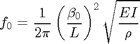
where is the elastic modulus, is the density, is the length,

is the area moment of inertia for the beam, is the diameter, and is a constant. This can be rearranged:

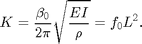
Then the fractional error in K,

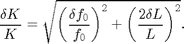
Determining the exact fractional error in a frequency measurement using the FFT is difficult, but it is almost always as good as 2/N, where N is the number of points in the time series. For the photogate we have N=768 so 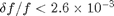. So the error will be dominated by until . If we have a ruler with and uncertainty of +/- 0.5 mm then we need or about 15 inches. From numeric simulation we can estimating the fractional error in frequency for a 50 count amplitude signal with negligible clock error and 768 samples to be . Thus the design goal from this analysis is that we should make the cantilever as long as possible.

However there are other considerations. For example, the equation is for a slender rod. So the diameter must be small with respect to length. So we want D/L as small as possible. But if D/L is too small then the rod will bend under its own weight. The deflection of a cylindrical cantilever under its own weight is given by:

The deflection must also be small for the equation to hold so L/D cannot be too large. The design criterion from these two equations and the slender assumption is that we want L/D to be as large as possible and

Then the final criterion can be stated as we want

as large as possible. There are other criterion like the density should be uniform, the cross-sectional area is constant, the material can not deform (like copper wire). However, this should give you and idea of how to think about the criterion for the pendulum you need from the theory section below. Since you will be using the same frequency measurement system you can assume that the fractional error in the frequency is . Make a list of your criterion to include in the report and to use in part II.

Theory of Pendulum

[0] Simple Pendulum: The simple pendulum consists of a massless[1] infinitely stiff rod[5] of length L and a point mass[1] m at the end in a uniform gravitational field with acceleration g. The rod is fixed at one end with a frictionless pivot[4] and the mass is at the other end and both are confined to move in a 2D plane[3] in a vaccuum[4]. The major approximations are in italics and numbered[#]. The frequency for small amplitude[2] osculations of a simple pendulum is:

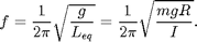
[1] Physical Pendulum: The physical pendulum relaxes the constraints [1] on the mass distribution. The main difference is that the equivalent length is given by , where I is the moment of inertial about the pivot and R is the distance from the pivot to the center of mass. So for a point mass and massless rod , and . This type of pendulum is also called compound which emphasizes that the parallel axis theorem can be used to build up the moment of inertial from the parts. A common example is the massive rod with a spherical mass at the end. You can use the parallel axis theorem to find I and the center of mass. Then the frequecy for small amplitude[2] oscillations of a physical pendlum is:

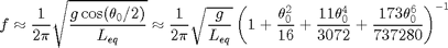
[2] Large Oscillation Pendulum: If we relax the constraint of small oscillations then the frequency is effected. To get the full solution we need to use elliptic integrals. There are also approximations that are quite accurate. See Richard B. Kidd and Stuart L. Fogg , A simple formula for the large-angle pendulum period , The Physics Teacher 40 , 81-83 (2002) [ doi ] [ pdf ]. Note that the following approximate formulas will work for a large initial angle in a physical (or simple) pendulum:

[3] Spherical Pendulum: If we relax the confinement of the pendulum to a 2D plane for example in a pendulum on a fixed length string then there is another angle for the pendulum to swing in. The period of the motion in is determined from angular momentum conservation (see. Conical Pendulum for the extreme cass of stationary . The previous formulas all work for this case as long as the angular momentum is zero. In practice, due to damping the angular moment will tend to zero. So if you start with a small rotation then it will damp away leaving pure in plane motion.

[4] Frictional Pendulum: Friction is present in all real pendulums. There are two main sources: frictional torque at the pivot and air resistance from the cross-sectional area of the pendulum in the direction of motion. A nice analysis of air drag is found here: Mohazzabi, P. and Shankar, S. (2017) Damping of a Simple Pendulum Due to Drag on Its String. Journal of Applied Mathematics and Physics, 5, 122-130 [ doi ] [ link ] [ pdf ]. The main point is that you need to reduce friction sufficiently so that your pendulum will swing for many oscillations. Ideally it would swing 20-30 times without much loss as our previous assumption that the fractional frequency error is is based on 25 consistent oscillations. Generally friction lengthens the period and therefore decreases the frequency.

[5] Elastic Pendulum: If the rod or string of a pendulum is elastic like a spring or rubber band then the motion can be very complicated and chaotic. If we had done a 6th lab we would have explored the motion of a weight on a rubber band being driven to choas. To measure gravity we need the pendulum to resist stretching. So a rubber band is not appropriate. However, for small oscillations the effect of stretching is usually negligible. For small oscillations the equations are linear so to a good approximation we can just add the solutions to each problem. The frequency of a mass on a spring with spring constant K is 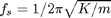. As long as then you should be ok.

Part II Experiment

From the theory above in Part I you have made a list of criterion. For the Cantilever experiment one of the main criteria was that we wanted the largest

we could find. For part II look around your house or work and try to find the best materials that will match your criterion. If needed you could buy a few things, but do not spend more than $10. For the cantilever experiment, I found that the Q for spaghetti was larger than most of the common materials in my house that came in a cylindrical form. Two other item had higher Q, bamboo skewers and steel skewers for shish kabobs. However the bamboo skewers have a lot of damping; they would only produce 3-4 oscillations. The steel skewers actually performed better than spaghetti, but the frequencies are very high, which is good for errors but not as visually clear what is happening. They are very sharp and difficult to cut. So for the measurement of density using water displacement they were not useable. They are also much more expensive and do not come in different diameters. Another interesting thing that I found was that whole wheat spaghetti has much more damping than regular. This may be because it is not as homogeneous.

1) Make a list (to include in the report) of several possible pendulum designs and evaluate them base on your empiric criterion from part I and on any other criterion you find useful to choose a specific design. Simple is always a good design criterion. It is better to start simple and add complexity as you go. As an example my entire pendulum consists of only 4 parts. Make a written description of your design before you build it for inclusion in the report. If you want some feedback you could send the description to me (as long as it is not the last day).

2) Build and test your design. A good design will oscillate for 100s of periods before stopping. It will have something thin a the very bottom to easily pass through the photogate. You may need to adjust your design as you go. This is part of the experimental process. Write a description of your final design and explain any major changes from you draft design from earlier.

3) Measure : Measure the equivalent length for your pendulum. Take a picture of you pendulum to include in the report and describe how you determined using the picture or diagrams as needed. Record and report the value and uncertainty in the standard form. From and the frequency derive and expression for gravitational acceleration g including any corrections as need from the theory section. Record and report how the fractional uncertainty in g depends on the fractional uncertainties in f and L.

4) Measure the frequency of the oscillation by letting the pendulum swing through the photogate from the Vibrating Cantilever Laboratory. The technique is very similar. The main difference is that the oscillation frequency will be lower and will last significantly longer. To account for these changes you will not really need to make 10 measurements to find the best one. Start the pendulum swinging and then use PhotoGateOscilloscope.m to measure the light in the photogate. This is a newer version of PhotoGateOscilloscope.m which allows much longer acquisition times needed for this experiment. Note: delete any older versions before saving. The ino file for the arduino PhotoGateOscilloscope.ino is the same. A typical command would look like this:

[V,T,N]=PhotoGateOscilloscope('com5',1,80000);

Notice that the second argument is 1. That means only one acquisition of 768 points will be taken. The time between each of the 768 is from the third argument. This total acquisition will take 768*.08s = 61s or about a minute. You will need to adjust the timing to get at least 25 oscillations in one acquisition. You can estimate the period of the oscillation from the known value of gravity. Remember that if the oscillations are larger than the size of the photoresistor there will be an apparent frequency doubling as the pendulum swings through from right to left and then again from left to right. If the amplitude is small enough then the pendulum will stay inside the photogate the whole time and the frequency will not be doubled. More typically there will be some power in both frequencies f and 2f. To measure the frequency you can use intFFT.m from the cantilever lab. A typical command would look like this:

[FV,f,f0]=intFFT(V,T,1000);
plot(f,FV);

From the plot you can zoom in to measure the peak frequency. With an interpolation of 1000 as above you will get 4 or 5 significant figures. If you need more you can increase to 10000 but it will take significantly longer and you will have to find the peak by searching through the values of FV. If you find that the peak is at index ii, then f(ii) is the corresponding frequency. The follow commands can automate the process if the peak you want is the largest:

[~,ii]=max(FV(1:N/2-1)); % find the location of the max of FV in the 1st half
f(ii)                    % f(ii) is the corresponding freq (ignore negative)

This method is not fool proof the frequency you want may not be the largest. If not you could use max on a different section of FV.

5) From the frequency and determine g. If it is within 10% you have a working gravity meter. If the error is greater than 1% see if there are any small modifications that you could do to improve. Once you are satisfied make 10 measurement of the frequency at the smallest amplitude where you can still get 25 good oscillations. Record and report the mean and std of the 10 measurements then calculate your best value of g in standard form with error estimate. Also record and report the deviation from the accepted value of 9.802 m/s/s (NYC). Is the deviation consistent with the error estimate?

Part III Proposal

Write a 1 paragraph proposal on how you could make the experiment more accurate if you could spend up to 100 dollars. How would you get the most accuracy with the fewest dollars. Include an estimate of the improved accuracy. You can assume that the frequency measurement has a fractional accuracy of which is relatively easy to get by collecting longer data sets. Since we are not measuring at full speed we can take very long data sets if needed.

Files

Published with MATLAB® 7.14