Vibration of a Cantilever
In this lab you will measure the vibration frequencies of a cantilever and determine the dependency on length and diameter.
- [ SPVib.pdf ] pdf version.
- [ SPVib.html ] html version.
https://www.vibrationdata.com/tutorials2/beam.pdf
Contents
Materials and Equipment
For this lab you will need:
- Three (3) boxes of dried spaghetti (cylindrical pasta).
- Each box should be a different known diameter.
- You should have previously measured the diameter and density of each type. If not see Density of Spaghetti Lab.
- NOT WHOLE WHEAT or WHOLE GRAIN!
- A ruler at least 12 inches with 1/16 inch rules or at least 30cm with at least 1mm rules. Example from amazon.
- Parts for an electronic photo-gate
(All
parts can be found in the LAVFIN kit from amazon.):
- Arduino Uno.
- Breadboard.
- Bright while LED.
- Photoresistor.
- 100 Ω and 1K resistors.
- Jumper wires.
-
1 clothes pin (Example)
- Must be spring loaded.
- Wooden ones work better.
- Other clamping devices could be used.
- Computer with free USB port for arduino.
- MATLAB.
- Technically not required, but would be more difficult without.
Building the Cantilever
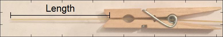
A cantilever is an elastic beam that is supported at only one end. The support limits movement and the angle. Mathematically, the cantilever can be described by a function Y(x) that varies along the length of the beam in x from 0 to L. At the fixed end, Y(0)=0 and Y'(0)=0. To achieve this boundary condition we need a clamp. A wooden clothes pin, as shown in figures 1 and 4, works well. Although other things could be used. The key is that the beam is fixed and cannot bend at one end. Typically you need at least 1cm in the clothes pin jaw to maintain these conditions. The cantilevers length is measured from the jaw (figure. 1).
Building Electronic Photo-Gate
In this section you will construct an electronic photo-gate. The gate will consist of an LED and a photoresistor. The light from the LED shines on the photoresistor. If anything enters the space between them, then the light on the photoresistor will decrease, which can then be measured as a voltage drop across a 1K resistor in series. (Note: This is a similar setup to lab II from PHYS 371.)
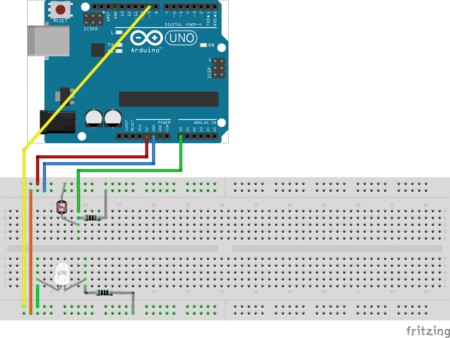
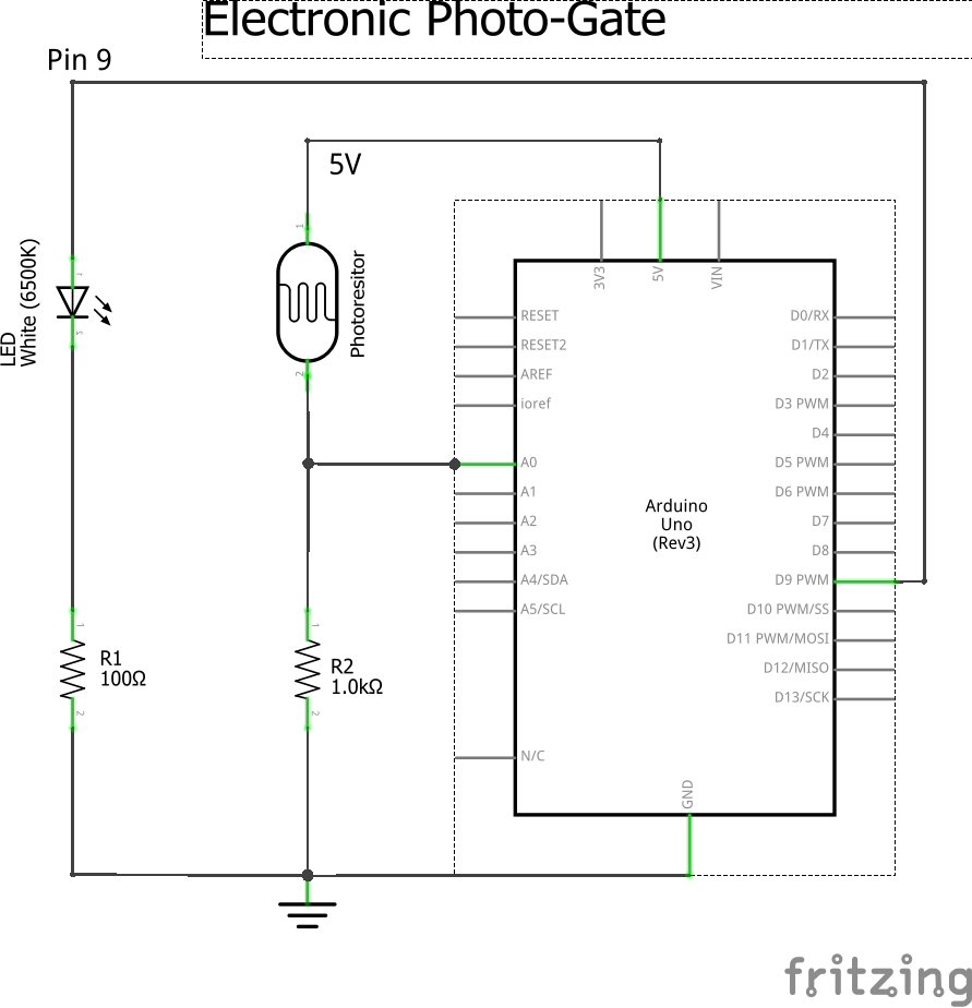
1) Build the photo-gate as described in figures 2-4. Details:
- Build the photo-gate as near to the end as possible so that the cantilever can extend beyond the breadboard and not hit it when vibrating.
- Make sure all of the wires are long enough to be pulled out of the way.
- Make sure to check the polarity of the LED.
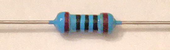
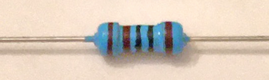
- High resolution photos of 100 ohm and 1K resistors are in figure 5.
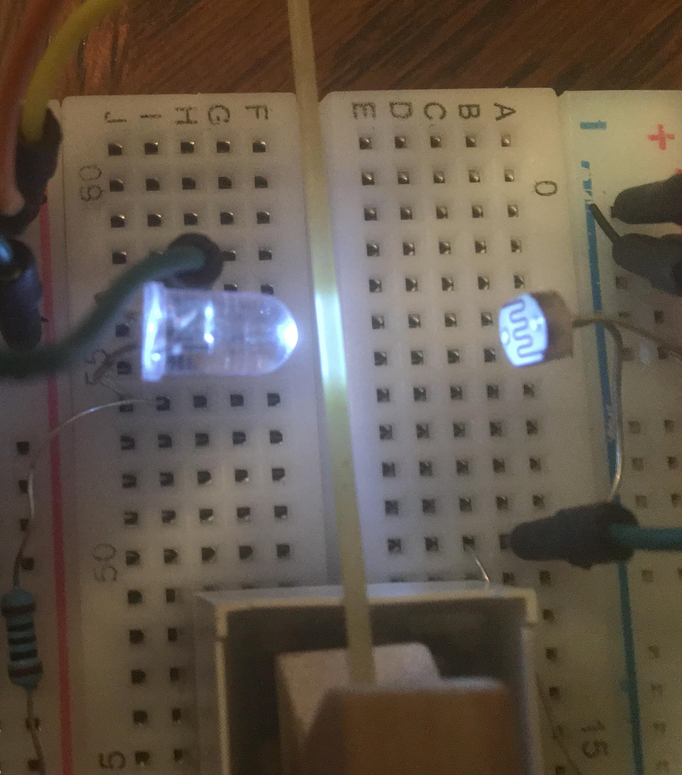
- The photoresistor should be oriented so that the wiggles are up and down. (See figure 6.)
Testing Electronic Photo-Gate
1) Connect the Arduino to your computer.
2) Download SimpleGate.ino (Right-Click: save link as or click through and copy/paste into an empty sketch).
3) Open the ino file in the arduino IDE, compile, and upload to the Arduino.
- You will not need to edit the code.
- There are comments if you are interested in how it works.
4) Trouble shoot the LED circuit:
- If everything is setup right the LED should turn on and the transmit light on the arduino should flash every second.
- If the LED is not on, but the transmit light is flashing then something is wrong with your LED circuit. Check each connection carefully. Pin 9 should be connected to the + side of the LED, the - side of the LED to 100 ohm resistor, and the resistor to ground. If you cannot get it working move on the the next step and come back once the A0 side is working.
- If the LED is not on, and the transmit light is NOT flashing, then the code did not get uploaded properly. Some things to try: 1) Upload Blink.ino. 2) Unplug the arduino, wait 30 sec and plug back in. 3) Reboot your computer. 4) And try again.
5) Trouble shoot the photoresistor circuit:
- Open the serial monitor and change the baud rate to 115200. This sketch uses a fast baud rate to speed up transfers.
- Once the baud rate is set you should see something like this:
Counts = 246 => 1.201V
Counts = 754 => 3.682V
Counts = 754 => 3.682V
Counts = 754 => 3.682V
Counts = 754 => 3.682V
Counts = 754 => 3.682V
Counts = 754 => 3.682V
- If you see this then, the sketch is working.
- If the value is zero, then A0 is likely connected to GND.
- If the value is wildly fluctuating, then A0 is likely not connected.
- Place an object between the LED and photoresistor and note the response on the serial monitor.
- With the gate clear you should get 700 to 800 counts or 3.4V - 3.9V.
- With an object in the gate the value should be lower. If it is higher, then your resistor and photoresistor may be reversed. It should be 5V to photoresistor, then 1K resistor to GND.
6) Optimize the photo-gate:
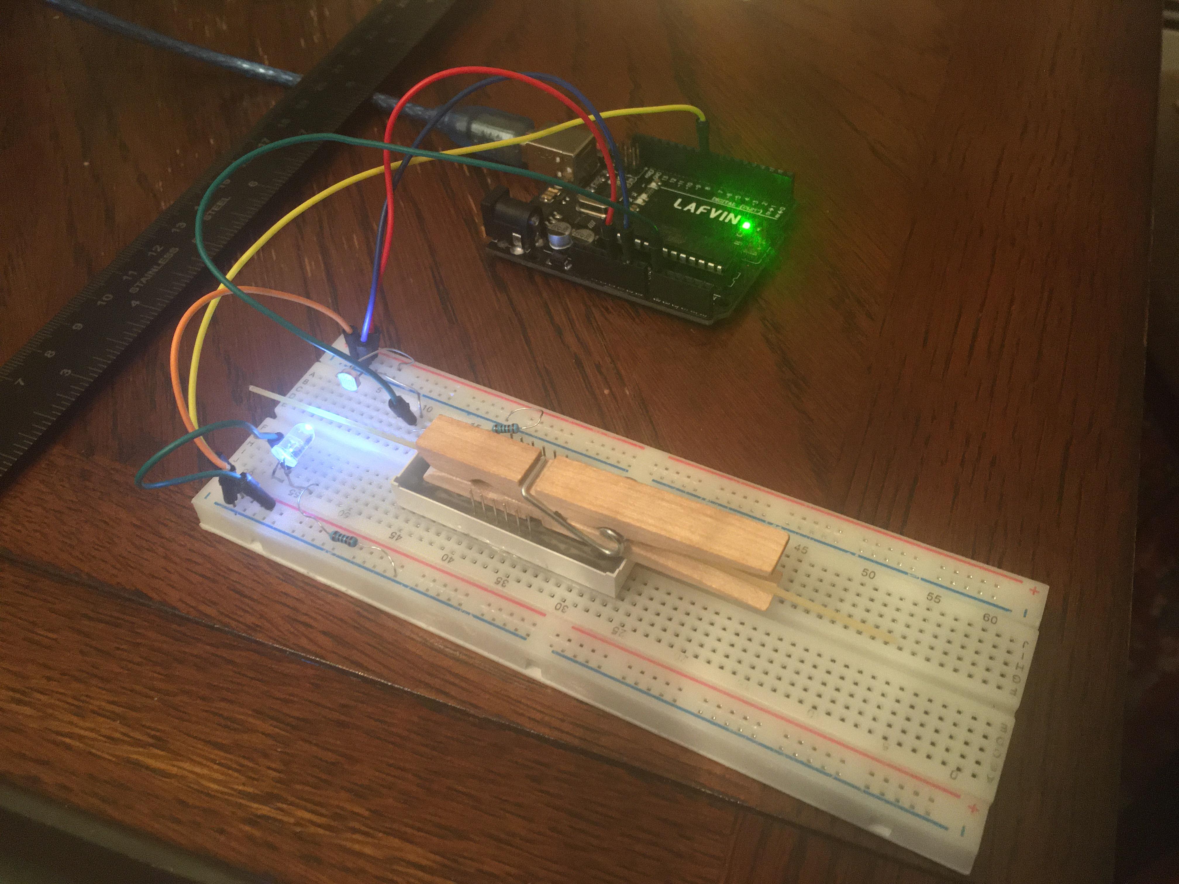
- Next place the cantilever with a strand of spaghetti on the breadboard. You may need to adjust the height of the cantilever to allow it vibrate without hitting the breadboard. I found that the 4 digit 7 segment display from the LAFVIN kit was just the right height when sitting upside down (see figure 7). Removing one wooden side from another clothes pin also worked well.
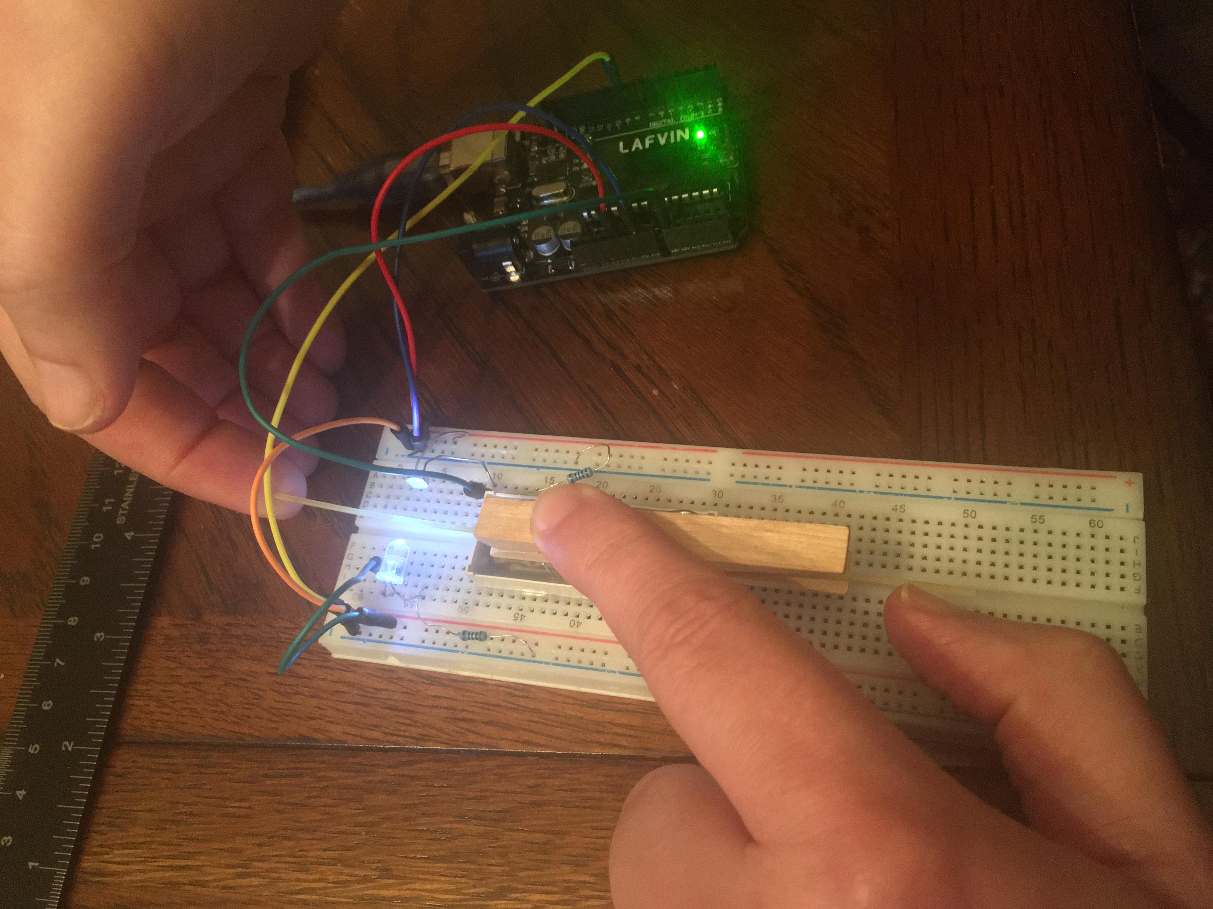
- Once the cantilever height is adjusted, place the jaws of the clothes pin about 1-2cm from the LED as shown in figures 7. Then bend the LED so that the light is pointing level and its center is at the height of the spaghetti.
- Now remove the cantilever and adjust the height and orientation of the photoresistor to get the largest open gate value.
- If you cannot get near 700 then you may have the wrong resistor.
- Now place the cantilever back in the middle of the gate. You should be able to see the shadow of the spaghetti on the photoresistor. Ideally, the shadow should be right across the wiggles on the photoresistor (see figure 8).
- Continue adjusting the LED and photoresistor until the open gate is between 700 and 800 and there is at least a difference of 50-100 when the spaghetti is in the gate. The difference is the most important.

8) After you have the gate optimized. Record and report the open gate reading.
9) Record and report the typical low reading with the spaghetti in the gate. Repeat for each of the 3 sizes of spaghetti. Do the low readings make sense? Explain.
10) If you are still having trouble with the LED you can use the A0 wire like a voltmeter and check the voltages in the circuit. Do you have 5V on the + side of the LED, etc?
Photo-Gate Oscilloscope
Now you will measure the time dependence of the light in the gate.
1) Download PhotoGateOscilloscope.ino (Right-Click: save link as or click through and copy/paste into an empty sketch).
2) Open the ino file in the arduino IDE, compile, and upload to the Arduino.
- You can ignore the low memory warning.
- You will not need to edit the code.
- There are comments if you are interested in how it works.
3) Manually test the sketch.
- Open the serial monitor and change the baud rate to 115200. This sketch uses a fast baud rate to speed up transfers.
- Type just the character '?' (no quotes) into the input area. The serial monitor should respond with the letter 'K' and turn up the brightness of the LED and light up the onboard LED.
- Now type 'g4000' (no quotes) in the input area. The arduino should take 768 voltage measurement at a rate of 1 per 4000us. You should see something like this:
667
667
667
667
667
667
667
667
667
667
3072120
- The last line is the total acquisition time approximately 768*4000=3072000.
- Now get ready to pluck the cantilever (see figure 7). Clear the monitor. Type in 'g4000' press enter and pluck the cantilever as quickly as you can. If you got the timing right you can scroll up and see some oscillation, like these:
739
688
735
685
732
692
733
691
726
702
722
700
- If you want you can plot them using favorite program. Here is mine:
makeFig(1);
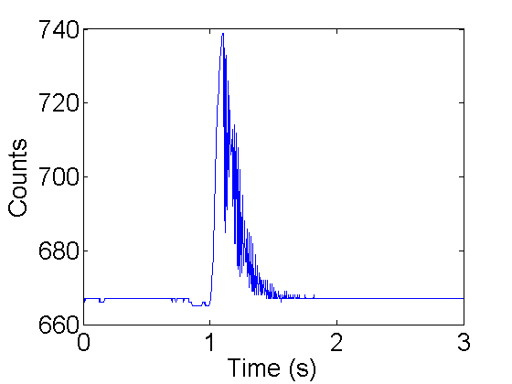
Figure 9. Counts vs time for manual vibration.
Automate using MATLAB
It might be possible to do all the measurement manually as you did in the previous section. (If you want to try, then contact Professor Shattuck for some hints.) However, it will be much easier to use MATLAB to automate things.
1) Download PhotoGateOscilloscope.m.
- PhotoGateOscilloscope is a function which returns time series from the photo-gate. It requires 1 input---the com port for your arduino. You can find the com port in the arduino IDE. The port name will will be listed on the tools menu. Mine is 'com5'. Here is a call to PhotoGateOscilloscope.
[V,T,N]=PhotoGateOscilloscope('com5');
size(V)
size(T)
disp(T);
disp(N);
ans =
     1   768
ans =
     1     1
     3072116
   768
This funtion returned V a 1x768 array (plotted above) which contains the voltage counts over time. The default acquisition time is 1 point per 120us. T holds the actual total acquisition time, and N is the number of points taken.
There are several other inputs that PhotoGateOscilloscope can take. A general call looks like this:
[V,T,N]=PhotoGateOscilloscope(port,M,dt,pauseit,plotit);
- port (required) com port for arduino
- M (optional default:1) Number of time series
- dt (optional default:0) Sample time in
 (minimum actual sample time 120us)
 - pauseit (optional default:false) true/false pause between acquisitions
- plotit (optional default:true) true/false plot data between acquisitions
Example I
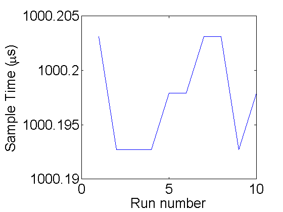
Here is an example plucking a 54.0 +/- 0.2 mm cantilever 10 times using the command:
[V,T,N]=PhotoGateOscilloscope('com5',10,1000);
In this example the sample time is set to 1000us. The actual sample time (T/N) looks like this:
load ex1;  % same as running: [V,T,N]=PhotoGateOscilloscope('com5',10,1000);
plot(T/N);
ylabel('Sample Time (\mus)');
xlabel('Run number');
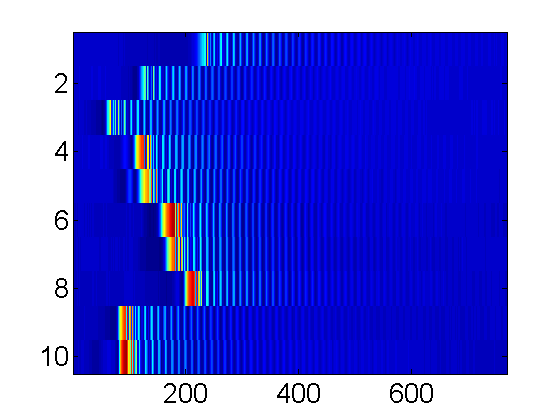
A quick way to look at all of the data is showing all 10 runs as an image where the y-axis is the run number and the x-axis is time step. The color of the image is determined by the count value:
colormap(jet(256)); % The best color map high to low:Red-Green-Blue
imagesc(V);         % display image
colorbar;           % show the value for each color
xlabel('Time (steps) (1-768)');
ylabel('Run number');
hold on;
plot(330,1,'w*',650,1,'wx','markersize',13,'linewidth',2);
set(gca,'xtick',[1 200 330 500 650 N]);
set(gca,'ytick',1:10);
hold off;
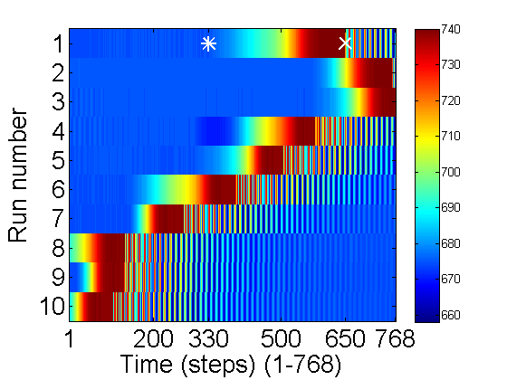
A few things to notice. The total range of dark to light is 660-740. Examine run 1: At the beginning of the run the cantilever was in the middle blocking the light so the count is low (~670). Then it was pulled up starting from time 330(*) to 650(x). Then it begins to oscillate, but the sample ends before it rings down. To check things more carefully lets plot the first run:
k=1; % set run number
% plot the k-th (1st) run. Add line at special times 330 and 650
plot(1:N,V(k,:),330*[1 1],[650 680],650*[1 1],[650 740],'linewidth',2);
xlabel('Sample number');
ylabel('Count');
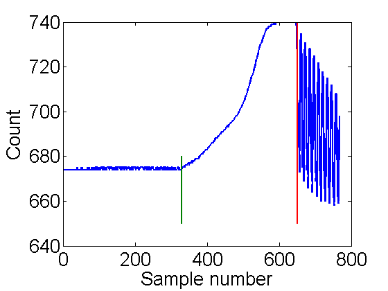
This confirms the description above. Here is a zoom in on the vibrations:
k=1; % set run number
% plot the k-th (1st) run. Zoom in to 650:end
plot(1:N,V(k,:),330*[1 1],[650 680],650*[1 1],[650 740],'linewidth',2);
peaks=654+(0:12.1:6*12); % mark strange peaks
text(peaks,V(k,fix(peaks)),sprintfc('%d',1:6),'vertical','bottom','horiz','center');
axis([650 N 650 740]);
xlabel('Sample number');
ylabel('Count');
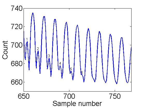
Notice the first 6 oscillations. There are strange peaks where there should be valleys. At 650 the cantilever was released above the gate. It is going down rapidly as it reenters the gate. Then the counts start going back up. This is due to the fact that the cantilever has left the gate through the bottom. Then at peak 1 it turns around and starts reentering the gate from the bottom. This causes an apparent frequency doubling, which is not present in the actual motion. When you take your data you need to be careful to limit this frequency doubling behavior. This example is OK. The correct frequency is dominate. Some things to try if it is too large:
- Slide clothes pin closer to the gate. (But not too close!) If you go too close then there will be no moving parts in the gate.
- Slightly raise or lower the cantilever. A few pieces of paper work well.
- Change the angle of the cantilever.
- Move closer to the LED. (But not too close!)
- Give a smaller pluck. (But not too small!)
Now returning to the whole set:
colormap(jet(256)); % The best color map high to low:Red-Green-Blue
imagesc(V);         % display image
colorbar;           % show the value for each color
xlabel('Time (steps) (1-768)');
ylabel('Run number');
hold on;
plot(330,1,'w*',650,1,'wx','markersize',13,'linewidth',2);
set(gca,'xtick',[1 200 330 500 650 N]);
set(gca,'ytick',1:10);
hold off;

For the first 7 runs the pluck came too late. (It takes a bit of practice to get the timing right). Some oscillations are lost off the end. However the last 3 look good. Let us examine the 10th one in more detail.
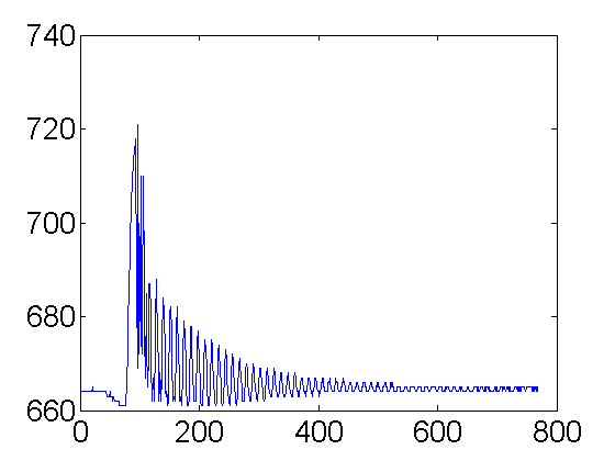
k=10;                            % plot the k-th (10th) run.
plot((0:N-1)*T(k)/N/1e6,V(k,:)); % command to plot one run against time (s)
xlabel('Counts');
xlabel('Time (s)');
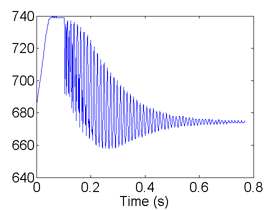
Right after the release at ~ 0.1s the frequency doubling is present, but should be ok for this run. Focus on the plotting command:
plot((0:N-1)/N*T(k)/1e6,V(k,:));
The time in seconds is determined by making a list from 0 to N-1 (0:N-1). Then multiply by the time per sample T(k)/N. T(k) is the total time for run k and N is the number of samples. Finally since T(k) is in dividing by 1e6 converts to seconds. V(k,:) is matlab for all (:) of the points in the kth run. This run looks good so lets analyze it.
One way to get the frequency is to zoom in and measure the peak-to-peak time difference. For example:
k=10;                     % plot the k-th (10th) run.
peaks=[250 298];          % peak positions
plot(1:N,V(k,:));         % command to plot one run sample number
hold on;
plot(peaks,V(k,peaks),'r.','markersize',20);   % plot peaks
axis([245 303 650 720]);
props={'vertical','bottom','horiz','center'};
text(peaks,V(k,peaks),sprintfc('(%d,%d)',[peaks;V(k,peaks)]'),props{:});
ylabel('Counts');
xlabel('Time (s)');
hold off;
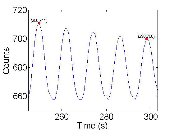
From this plot, 4 cycles took:
S=298-250;  % steps between peaks
dS=0.5;     % uncertainty in peak position 1/2 step
fprintf('S=%3.1f +/- %3.1f Steps',S,dS);
S=48.0 +/- 0.5 Steps
To get the frequency:
S1=S/4;        % steps for 1 cycle
T1=S1*T(k)/N;  % period in us => steps/period * time/step
T1s=T1/1e6;    % period in s => us * s/(1e6 us)
fs=1/T1s;      % frequency = 1/period

% All in one equation:

f1=1/((S)/4*T(k)/N/1e6);

% Most of the numbers in this equation are exact, except for S and T(k), however
% T(k) is very accurate so the error in T(k) can be ignored.  A quick way to get
% the error is to evaluate |f1(S-dS)-f1(S+dS)|/2.  This is only easier because
% there is only one uncertain variable:

df1=abs(1/((S-dS)/4*T(k)/N/1e6)-1/((S+dS)/4*T(k)/N/1e6))/2;
fprintf('f=%3.1f +/- %3.1f Hz',f1,df1);
f=83.3 +/- 0.9 Hz
How could this measurement be improved?
Another technique to extract the frequency is to use the Discrete Fourier Transform (DFT). The DFT gives the amount of each frequency in a time signal. For periodic data we should see a few peaks. To use the DFT the frequency bandwidth must be extracted from the time series. The bandwidth is the size of frequency domain. It is determined from the sampling frequency. The sampling frequency is equal to the total bandwidth. It seems clear that we cannot understand anything about frequencies that are larger than our sampling frequency. For this example the sampling period is very close to 1000 = 1ms = 1/1000 seconds so the sampling frequency is 1/(1/1000) or 1000Hz. So we should not expect to gain any information about frequency >1000Hz. However, it is worse than that. We need 1/2 the band width to distinguish (+) frequencies from (-) so the maximum frequency that can be measured with a 1000Hz sample frequency is 500Hz. Another way to see the factor of 2 is that it take 2 samples per period to measure a frequency.
To see how use the DFT in matlab, we can break it down in steps:
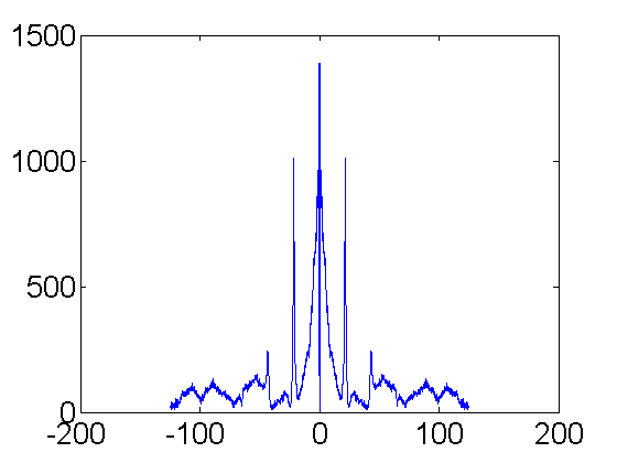
f0=N/T(k)/1e-6;   % calculate the sample frequency
n=(-N/2:N/2-1)/N; % Make a list that goes from -1/2 to 1/2-1/N in N steps.
                  % The weird 1/N is because we have an even N.
f=f0*n;    % The whole range is ~1 so multiply by f0 to get full bandwidth

Vm=V(k,:)-mean(V(k,:)); % subtract mean to suppress zero freq component.
FV=fft(Vm);             % fft is the fast DFT.
FV=fftshift(FV);        % Put zero frequency in the middle (fyi:doc fftshift)
FV=abs(FV);             % DFT is complex so need modulus to easily view

plot(f,FV);               % plot the DFT
xlabel('frequency (Hz)'); % frequency band -500Hz to 500Hz or 1000Hz
ylabel('Amplitude');      % Relative amount of each frequency in the signal

set(gca,'xtick',[-500 -300 -100 0 100 300 500]);

peak=448;    % find peak near 80Hz from plot
text(f(peak),FV(peak)*1.05,num2str(f(peak)));

df=f0/2/N;   % error from frequency spacing
fprintf('f=%3.1f +/- %3.1f Hz',f(peak),df);
f=82.0 +/- 0.7 Hz
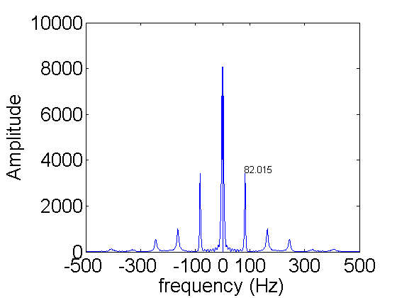
There are at least 11 peaks. For real data the DFT is symmetric around zero. So the negative frequency peaks do not give any new information. So that leaves 5 peaks. The one near zero frequency is the slow change from high to low over the whole acquisition. The peak at 82Hz is the natural frequency of the cantilever. The next peak at 164Hz is from the frequency doubling discussed earlier. Each of the higher peaks are a multiple of 82Hz. They are there because the oscillation is not a perfect sin or cos wave.
So both techniques are useful. In the time domain it is easy to see where the base frequency is so we can look in the right place. The frequency domain gives an overview of all of the relevant frequencies.
The frequency spacing in the frequency domain limits the accuracy. If we zoom in on the main peak, we see that it is hard to tell where the peak is exactly (blue curve).
k=10;
f0=N/T(k)/1e-6;
% short vesion
plot(f0*(-N/2:N/2-1)/N,abs(fftshift(fft(V(k,:)-mean(V(k,:))))),'o-','linewidth',2);
hold all;

R=10; % zerofill by 10 interpolation
f=f0*(-R*N/2:R*N/2-1)/N/R;
FV=abs(fftshift(fft([zeros(1,(R-1)*N) V(k,:)-mean(V(k,:))])));
plot(f,FV,'r.-');

xlabel('frequency (Hz)'); % frequency band -500Hz to 500Hz or 1000Hz
ylabel('Amplitude');      % Relative amount of each frequency in the signal
axis([78 86 0 4000]);     % zoom in
peak=4473;    % find peak near 80Hz from plot
text(f(peak),FV(peak)*1.05,num2str(f(peak)));
hold off;
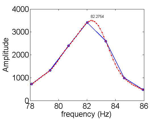
There is a nice way to interpolate DFTs, which is optimal for band limited signals. Band limited signals have no peaks outside of the bandwidth. Our DFT shows that the signal is dropping fast at high frequencies. Therefore we can use it to increase the accuracy. The simple formula is to add zeros to signal before using the fft (see the above code). The result of 10x interpolation is shown in red above. From the new peak we get a new estimate for the frequency. Why not keep interpolating? We cannot go on forever. To estimate the error using this technique depends on the signal-to-noise ratio and its calculation is beyond the scope of PHYS 471. You should be safe in dividing the error by 3 with a x10 interpolation. Here is the new result:
df=f0/2/N;   % error from frequency spacing
df=df/3;     % actual error is difficult to calculate a factor of 3 better is typical
fprintf('f=%3.1f +/- %3.1f Hz',f(peak),df);
f=82.3 +/- 0.2 Hz
Example II
The second example will go more quickly using the helper function intFFT.m. The function intFFT is a shortcut for calculating interpolated FFTs. The inputs and output are given here:
[FV,f,f0]=intFFT(V,T,R);
- FV is the interpolated DFT of V.
- f is the frequency list for a total sample time of T in .
- f0 is the sample bandwidth
- V is the time series to transform
- T is the total sample time in .
- R (optional: default:0) interpolating factor.
For this example, I have lengthened the cantilever by a factor of 2 to 108 +/- 0.4 mm. With a longer cantilever, we expect that the frequency wiil be lower. Here are the results from running the PhotoGateOscilloscope function;
[V,T,N]=PhotoGateOscilloscope('com5',10,4000);
load ex2; % same as running: [V,T,N]=PhotoGateOscilloscope('com5',10,4000);
imagesc(V);
From this I choose the 9th run.
k=9;
plot(V(k,:));
Some frequency doubling but not too bad.
[FV,f,f0]=intFFT(V(k,:),T(k),10);
plot(f,FV);
From the 10x interpolated fft, I find a peak frequency of 21.55 Hz.
fp=21.55;
df=f0/2/N/3;   % error from frequency spacing /3 from interp x10
fprintf('f=%3.1f +/- %3.1f Hz',fp,df);
f=21.6 +/- 0.1 Hz
Frequency vs. Length and Diameter
You will find the dependence of cantilever frequency on length and diameter.
1) For each of the 3 diameters of spaghetti measure the frequency of vibration for 8 lengths. They should be approximately 3cm to 24cm in steps of 3cm. I found it easiest to mark the strands for each length. The exact length do not matter, but you should use the same 8 lengths for each diameter.
To aid in you data storage you may want to create a 3 by 8 by N=768 array to store your best time-series, and 4 3 by 8 arrays to store your lengths, diameters, frequencies, and acquisition times. For example:
allV=zeros(3,8,N); % create time series array once then fill as data is collected
allL=zeros(3,8);   % create Length array once then fill as data is collected
allD=zeros(3,8);   % create Diameter array once then fill as data is collected
allf=zeros(3,8);   % create Diameter array once then fill as data is collected
allT=zeros(3,8);   % create total time array once then fill as data is collected

%examples
allV(1,1,:)=V(k,:); % I choose k=9 for from this data for length 1 and diameter 1
allL(1,1)=104;      % length (mm) for length 1 diameter 1
allD(1,1)=0.85;     % Diameter (mm) for length 1 diameter 1
allf(1,1)=104.56;   % frequency (Hz) for length 1 diameter 1
allT(1,1)=T(k);     % Time for k=9 for diameter 1 length 1
You can also save the arrays:
save allV allV;
save allL allL;
save allD allD;
save allf allf;
save allT allT;
Or save them all together:
save alldata allV allL allD allf allT;
To retreive them later, for example:
load allV; % load saved V array
Exporting data to csv format.
- The first row will be the 24 L values.
- The second row will be the 24 D values.
- The third row will be the 24 T values.
- The forth row will be the 24 frequency values.
- Rows 5-5+768 will be the V data values.
% write all data to one file
dlmwrite('alldata.csv',[allL(:) allD(:) allT(:) allf(:) reshape(allV,24,N)]','precision','%f');
Or you could write the processed and raw data separately:
Processed data:
- The first row will be the 24 L values.
- The second row will be the 24 D values.
- The third row will be the 24 T values.
- The forth row will be the 24 frequency values.
Raw data:
- Rows 1-768 will be the V data values.
% write processed data to one file:
dlmwrite('procdata.csv',[allL(:) allD(:) allT(:) allf(:)]','precision','%f');

% write raw data to one file:
dlmwrite('rawdata.csv',reshape(allV,24,N)','precision','%f');
Any of these methods will also make it easy to turn in your raw data.
Data Analysis and Theory
Elasticity theory predicts the frequency of the n-th mode is given by:
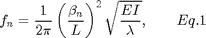
where  is the elastic modulus,
  is the mass per unit length,
  is the length,

is the area moment of inertia for the beam,  is the diameter, and
  is the nth zero of the equation:
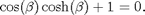
To get in MATLAB use the helper function betaN. For example, in our case we alway have the lowest mode n=1.
fprintf('beta=%f',betaN(1));
beta=1.875104
The mass per unit length
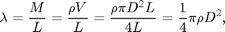
where  is the volume of the spaghetti strand and
  is the density measured in the Density of Spaghetti lab. Combining with the definition of
  and Eq. 1
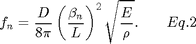
Thus the frequency is proportional to

with proportionality constant

Use your data to verify that is a constant for spaghetti cantilevers and report the value for in standard form from a loglog fit to Eq. 2. Explain how the uncertainty in was calculated.
Clean up
Save the spaghetti and photo-gate apparatus for a latter lab.
Files
- SPVib.zip All files in one zip file.
- SPVib.m (This File).
- SPVib.pdf (pdf version).
- PhotoGateOscilloscope.m Photo-gate acquisition function.
- intFFT.m Interpolated FFT.
- betaN.m Calculate .
- SimpleGate.ino
