Virtual Millikan Oil Drop
In this lab you will measure the charge of the electron and show that the charge is quantized using a virtual version of the famous Millikan oil drop experiment.
- [ VMOilDrop.pdf ] pdf version.
- [ VMOilDrop.html ] html version.
You should read the manual for the physical version of this experiment. The virtual version is based on this experiment. All of the physical data is take from there. You can use it like a manual for doing the experiment. This document will help set up the virtual version of the experiment, but the physical version should guide you as you perform the experiment. The example data at the end is particularly useful. The one issue in the physical manual is the hint from table 1.1. I think this data is probably for an electric field closer to 500V/cm instead of 1000V/cm.
Contents
Materials and Equipment
For this lab you will need:
- Parts for an voltage controller with separate magnitude,
ON/OFF, and polarity:
(All parts can be found in the LAVFIN
kit from amazon.)
- Arduino Uno.
- Breadboard.
- 10K Potentiometer.
- (3) push buttons.
- Jumper wires.
- Computer with free USB port for arduino.
- MATLAB.
- Stop watch (phone timer).
Experimental overview
We will create a virtual virtual version of the famous Millikan oil drop experiment. This experiment measured the value of the electron charge and demonstrated that every electron had the same charge. You will use the virtual version to accomplish the same goal. In this experiment, small  oil droplets are introduced into a thin air-filled chamber. The drops are exposed to ionizing radiation to add a net charge. Their fall under gravity can be observed through a small hole with a microscope. A controllable electric field pointing in the direction of gravity provides a second force on the drops. Depending on the field direction UP(+) or DOWN(-) the electric force can oppose or add to the gravitational force.
The mass of the particle can be determined from the terminal velocity of the falling droplet with the electric field off. (See Stokes drag law.) The density of the oil  determines the diameter of the falling drop. Applying an electric field
  changes the force on the drop with the addition of a term
  proportional to the charge
  . From the new terminal velocity in field , the value of can be measured. For a detail analysis see the experimental manual.
There are 5 controls for the experiment:
- Set Voltage magnitude: to set the electric field strength.
- Voltage Power: to turn the electric field on and off.
- Voltage Polarity: to set the electric field direction.
- Charge Reset: to change the charge on the droplets. In the experiment this is accomplished by exposure to ionizing radiation. In the virtual experiment the charge will be randomly changed at the push of a button.
- Spray new droplets: to get a new set of droplets. In the experiment there is an actual atomizer for the oil. In tht virtual experiment there will be an Exit function to stop and restart the simulation with a new set of drops.
For a shorthand in the virtual version each input will be referred to using the name in bold. We will simulate these controls using the Arduino as follows:
- Voltage: implemented using a 10K potentiometer.
- Power: implemented with a push button in ON/OFF toggle mode (on press).
- Polarity: implemented with a push button in (+)/(-) toggle mode (on press).
- Reset: implemented with a push button in one-off mode (on release).
- Exit: implemented reusing the Reset button in a push and hold mode.
This guide will walk you through the setup of the virtual experiment, but once built you will perform the experiment in the same way as the actual experiment, by measuring the velocity of droplets falling under various conditions: O) gravity alone field Off, U) gravity and field Up, and D) gravity and field Down. The velocity measurements will be made, just as I and so many other students before you have done, by timing the fall between two rules, as seen below:
Building the Virtual Millikan Oil Drop Experiment - Arduino control panel.
In this section we will build the Arduino portion of the experiment.
The ciruits for this lab can be built without interfering with the photogate from the previous lab, which we may use again in a later lab. Therefore the breadboard and schematics include all of the components for both labs. You can ignore the parts you already have.
We will construct some simple input devices that Matlab will use to control this virtual oil drops.
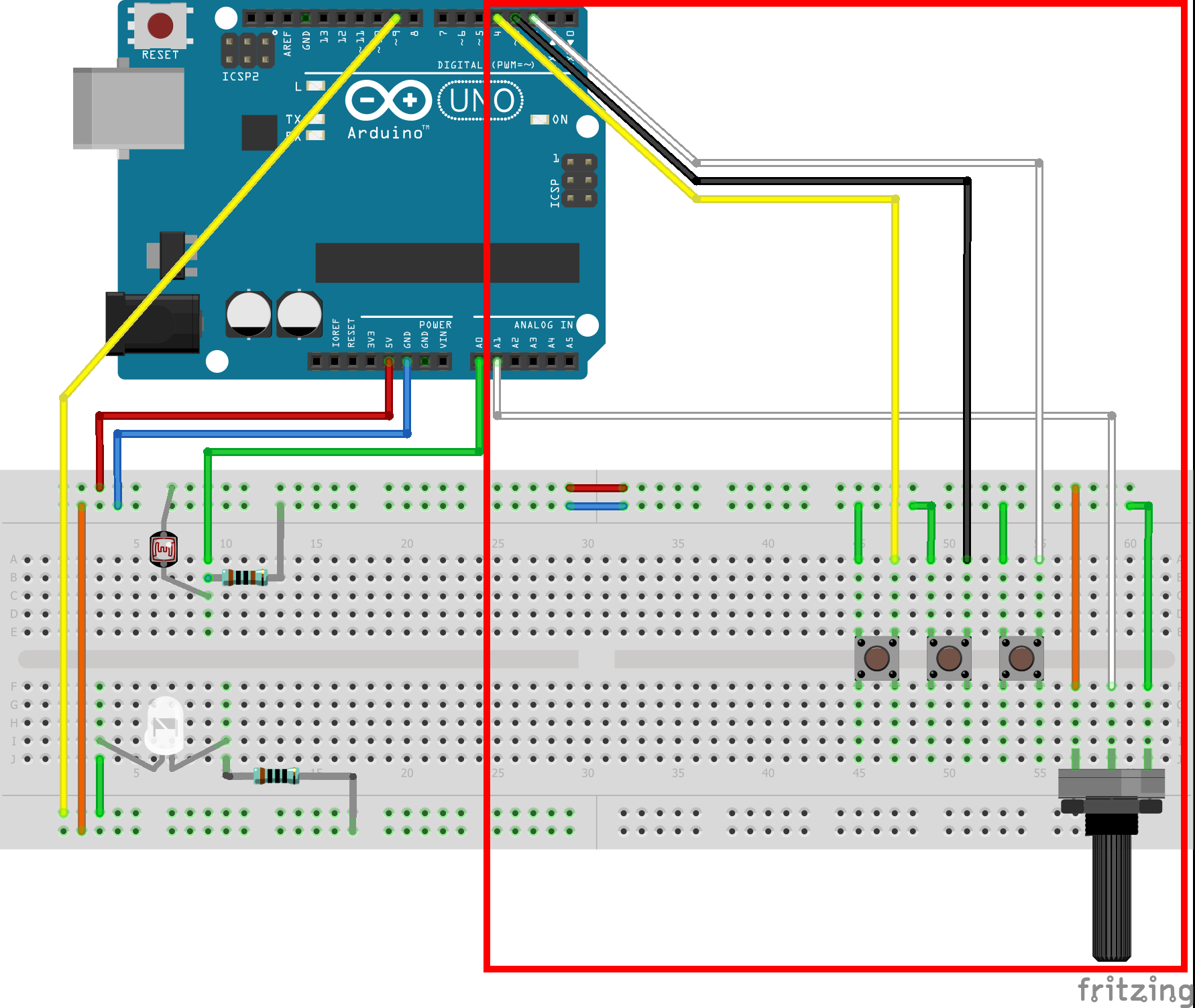
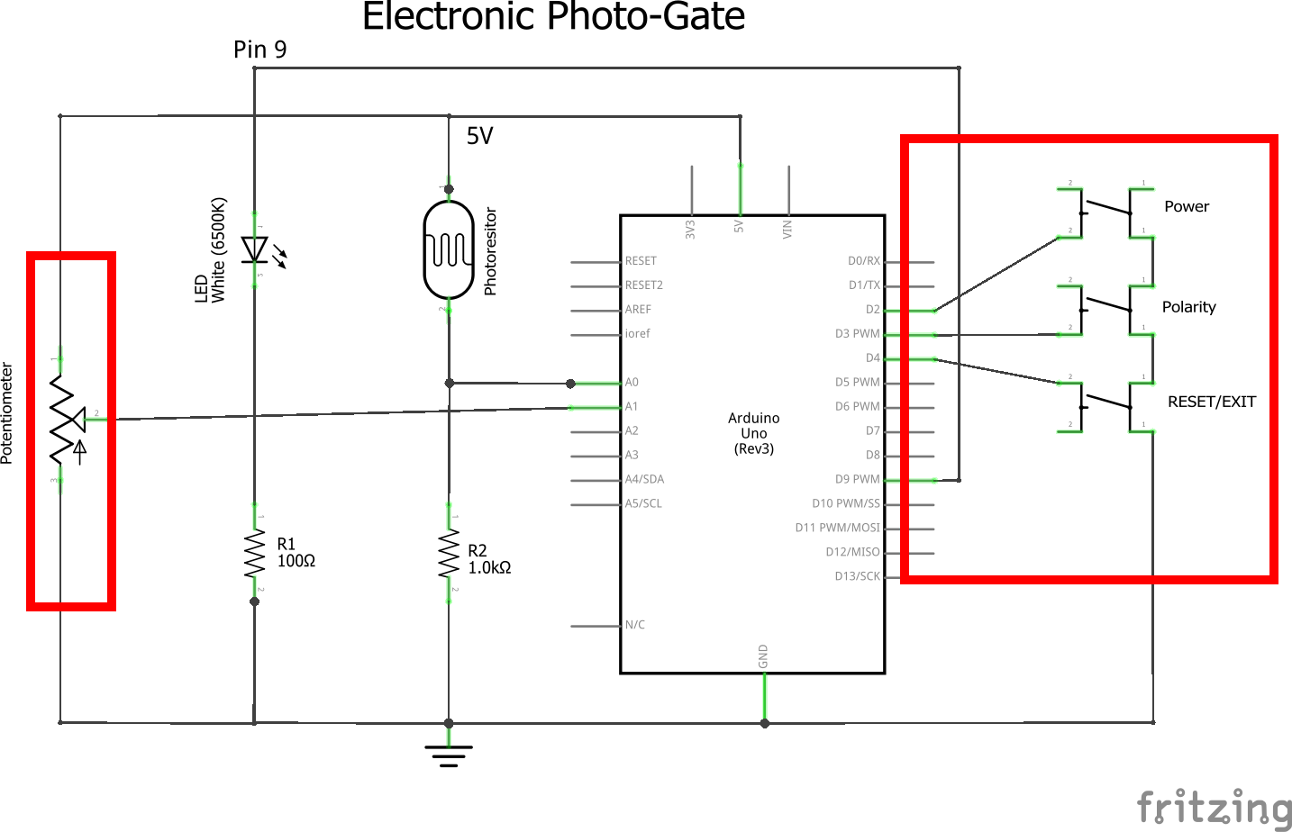
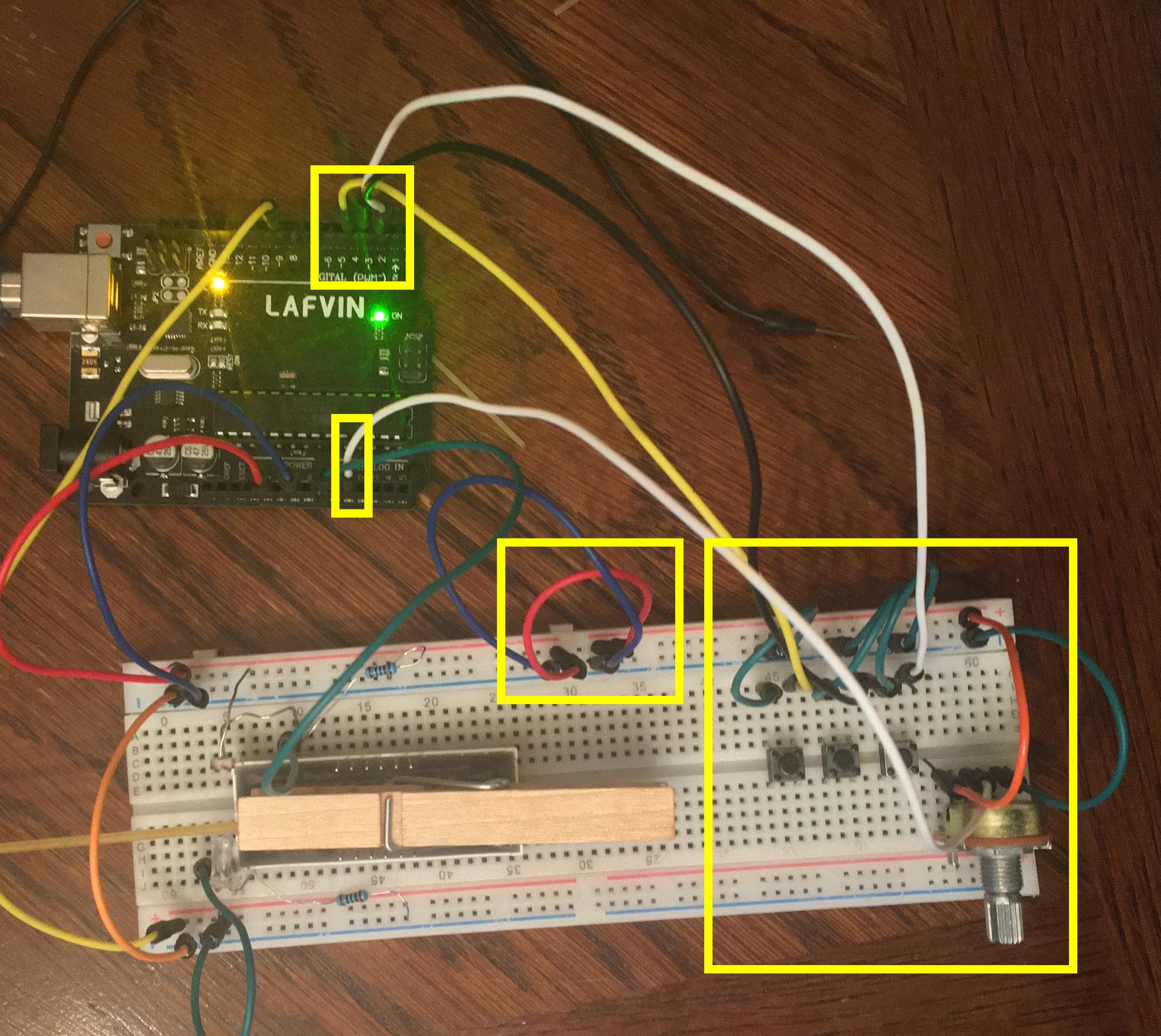
1) Build the Virtual Oil Drop input panel as described in figures 2-4. Details:
- Build the Virtual Oil Drop input panel as near to the end as possible so that it is out of the way of the photo-gate.
- Note: the blue and red connections between the two sides of the breadboard which bring +5V and ground from the existing circuits.
- The buttons are in order from closest to the potentiometer to furthest connected to digital inputs 2,3,4. These will correspond with Power (ON/OFF), Polarity (+)/(-), and Reset/Exit.
Testing Virtual Oil Drop input panel
1) Connect the Arduino to your computer.
2) Download VirtualOilDropPanelTest.ino (Right-Click: save link as or click through and copy/paste into an empty sketch).
3) Open the ino file in the arduino IDE, compile, and upload to the Arduino.
- You will not need to edit the code.
- There are comments if you are interested in how it works.
4) Open the serial monitor and change the baud rate to 115200. This sketch uses a fast baud rate to speed up transfers. Once the baud rate is set you should see something like this:
Voltage = 1023 power=OFF  polarity=(+)
Voltage = 1023 power=OFF  polarity=(+)
Voltage = 1023 power=OFF  polarity=(+)
Voltage = 1023 power=OFF  polarity=(+)
5) Turn the potentiometer and the Voltage should change. Note where the max of 1023 and min of 0 is found on the dial:
Voltage = 1023 power=OFF  polarity=(+)
Voltage = 1023 power=OFF  polarity=(+)
Voltage = 1023 power=OFF  polarity=(+)
Voltage = 716 power=OFF  polarity=(+)
Voltage = 523 power=OFF  polarity=(+)
Voltage = 54 power=OFF  polarity=(+)
Voltage = 0 power=OFF  polarity=(+)
Voltage = 181 power=OFF  polarity=(+)
Voltage = 555 power=OFF  polarity=(+)
Voltage = 363 power=OFF  polarity=(+)
Voltage = 322 power=OFF  polarity=(+)
Voltage = 912 power=OFF  polarity=(+)
6) Press the Power button. One press toggles ON and stays on. Next press back to off. Note the change should occur as you press not as you release:
Voltage = 1023 power=OFF  polarity=(+)
Voltage = 1023 power=OFF  polarity=(+)
Voltage = 1023 power= ON  polarity=(+)
Voltage = 1023 power= ON  polarity=(+)
Voltage = 1023 power=OFF  polarity=(+)
Voltage = 1023 power=OFF  polarity=(+)
Voltage = 1023 power= ON  polarity=(+)
Voltage = 1023 power= ON  polarity=(+)
7) Press the Polarity button. One press toggles (-) and stays (-). Next press back to (+). Note the change should occur as you press not as you release:
Voltage = 1023 power= ON  polarity=(+)
Voltage = 1023 power= ON  polarity=(+)
Voltage = 1023 power= ON  polarity=(-)
Voltage = 1023 power= ON  polarity=(-)
Voltage = 1023 power= ON  polarity=(+)
Voltage = 1023 power= ON  polarity=(+)
Voltage = 1023 power= ON  polarity=(-)
Voltage = 1023 power= ON  polarity=(-)
8) Press the Reset/Exit button. One press/release creates one and only one RESET signal. Press/release again for another RESET. Note the change should occur as you release not as you press. This is to accommodate a press/hold function to exit (see below):
Voltage = 1023 power= ON  polarity=(-)
Voltage = 1023 power= ON  polarity=(-)  RESET
Voltage = 1023 power= ON  polarity=(-)
Voltage = 1023 power= ON  polarity=(-)
Voltage = 1023 power= ON  polarity=(-)  RESET
Voltage = 1023 power= ON  polarity=(-)
9) Press and hold the Reset/Exit button. After holding for ~3 seconds the program should print EXIT and stop:
Voltage = 1023 power= ON  polarity=(-)
Voltage = 1023 power= ON  polarity=(-)
Voltage = 1023 power= ON  polarity=(-)  EXIT
10) If all of the above work you are all set.
11) Troubleshooting:
- If nothing changes the output then you should check you power connections. Make sure 5V and GND are connected from one side of the board to the other.
- If the potentiometer is not working or cannot create the whole range from 0-1023, check the pin order. In the picture from the edge of the breadboard the closest to the edge connects to GND; Next, in the middle connects to A1; Next connects to 5V. In fact the only one that really matters is the middle to A1. The GND and 5V could be switched and the 0 would just be on the other side.
- If the buttons are not working, check the orientation. The legs stick out on one pair of sides and not the other. The fact that they stick out gives them the distance to reach across the middle comfortably. In the other direction they skip one row. Make sure your connections skip. It does not matter which side is connected to GND and which to the digital inputs. You can right click and download figure 4 to zoom in if needed. The order of the buttons is also not critical, but I found the optimal for me was Power (D2), Polarity (D3), Reset/Exit (D4).
Virtual Oil Drop input panel
Now you test the sketch that will interface with matlab.
1) Download VirtualOilDropPanel.ino (Right-Click: save link as or click through and copy/paste into an empty sketch).
2) Open the ino file in the arduino IDE, compile, and upload to the Arduino.
- You will not need to edit the code.
- There are comments if you are interested in how it works.
3) Manually test the sketch.
- Open the serial monitor and change the baud rate to 115200. This sketch uses a fast baud rate to speed up transfers.
- Type just the character '?' (no quotes) into the input area. The serial monitor should respond with the letter 'K' and light up the on board LED.
- Now type 'g' (no quotes) in the input area. The arduino should repsond with something like the following:
K
3FF4
4) Each time you type 'g' (no quotes) another 2-4 character line will be printed. If you change the potentiometer or press the buttons the line will change. Here is the response to ?<cr>g<cr>g<cr> then turn dial, press a few buttons then g<cr> press another button g<cr>:
K
3FF4
3FF4
1D0C
1D08
Each line is a 2-4-byte hexadecimal number code. The first 1-3 bytes encode the 10-bit value of the potentiometer. The last byte is a bitmap for the button state of the form 0bXXXXWPRE with:
- W -> power state ON/OFF
- P -> popularity state 1=>(+) / 0=>(-1)
- R -> RESET state RESET/!RESET
- E -> EXIT state EXIT/!EXIT
- X -> Not used
If this is not meaningful to you, don't worry. I added it for those interested.
5) If your output looks similar to the above, then You are ready for Matlab.
Using the Virtual Millikan Oil Drop Experiment - Matlab
It will not be possible to do the lab without MATLAB.
1) Download VMOilExp.m.
- VMOilExp is a function which simulates a virtual oil drop experiment.
- A general call looks like this:
VMOilExp(port,demo);
- port (required) com port for arduino
- demo (optional default:false) true or false to put in demo mode
It requires 1 input---the com port for your arduino. You can find the com port in the arduino IDE. The port name will will be listed on the tools menu. Mine is 'com5'.
Demo Mode
To get started, run VMOilExp in demo mode:
- Create a docked figure window. The figure window needs to be docked to run properly in real-time. From the command window you can type:
h = figure;
set(h, 'WindowStyle', 'Docked');
- Resize the figure so it is square and covers 80-90% of your vertical screen. This is not required, but you will be visually making measurement in the figure window so it is recommended.
- Change to the directory where you downloaded the file VMOilExp.m and type the following command in the command window. (Note 'com5' should be replaced by your com port. See above.)
VMOilExp('com5',true);
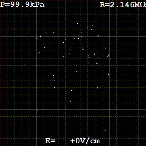
- You should see something like figure 5 below.
- Press and hold Reset/Exit until the program stops.
- If the program will not stop you can stop it with the stop execution command, ctrl-c (PC) or command+ (MAC). If you use this method you will need to manually close the serial port. To aid this process you can download closeAllPorts.m function to do it for you. The command can be run from the command line like this:
closeAllPorts()
- If the Exit button did not work check back over the previous sections to make sure it is working in the serial monitor. The 2-4-byte hex code for EXIT will be odd if Exit was recognized. Odd hex numbers end 1,3,5,7,9,B,D,F.
- If everything worked get ready for the last test: Timing the fall of the drops in demo mode. Use a stop watch or phone timer to measure the time it takes one of the drops to fall from one major rule to the next. It should take 20 seconds. To restart the virtual oil drops in demo mode press and hold Reset/Exit until it stops, then type the following in the command window:
VMOilExp('com5',true);
- If the time is close to 20 seconds then everything is working now. Use the demo mode to practice timing and get a feel for how many measurements are needed to get an accurate velocity. Record and report the velocity you measured in standard form with error estimates for the demo mode velocity. What is the percent deviation from the accepted value of:
- If you do not get something close to 20 seconds then let Professor Shattuck know so we can debug the problem.
The Virtual Millikan Oil Drop Experiment
Now you are ready to perform the actual experiment following the instructions for the physical lab. Several notes:
- You can now run the non-demo mode version by typing the following command into the command window:
VMOilExp('com5');
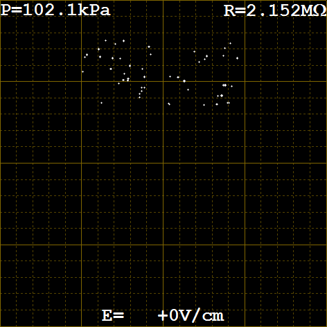
- Controlling the Electric Field: When virtual experiment starts the Power is OFF so the electric field is off and the drops will fall. The current magnitude and polarity of the field are shown at the bottom of the screen. When it starts, it should read +0V/cm, which means the Polarity is (+) and the Power is OFF. The current value of the Voltage is not displayed when the Power is OFF. If you turn the Power ON then the electric field magnitude and direction will be shown. If you have the Voltage at max 1023 then the field will show +1023V/cm, and most of the drops will start to rise. There is a chance they have no net charge and the electric field will not effect them. If you press the Polarity button the field will flip and now will read -1023V/cm. All of the drops will fall now. Some very fast if they have a high charge. If you now press the Power button then the field will read -0V/cm. Indicating that the field is off, but it will be in the downward direction (-) if turned on.
- Manipulating the particles: Using combinations of the Voltage nob, the Power button, and the Polarity button you will be able to control the positions of the drops. You can manuver specific drops to fall past the major rules and measure their velocities. With the Power ON and Polarity (+) they will move up (if the field is strong enough and they are charged). You can measure their upward velocity. Then flipping the polarity or turning the Power OFF they will fall again for you to repeat the process. I found a good cycle was to measure fall rate at +0V/cm, then Power ON at +500V/cm to measure upward velocity, then repeat. Then periodically replace the fall at +0V/cm with a faster fall at -500V/cm. But whatever order you choose is fine.
- Restart: You can keep the simulation running indefinitely, but it requires input to keep the particles on the screen. When you have lost all of the drops or want to stop, press and hold the Reset/Exit button. When you restart the particles will have new diameters, new charges, and start near the top of the screen. In the physical experiment this corresponds to rotating the radiation source and squeezing the atomizer.
- Selecting a good particle: To make a good measurement you need to make many measurements on the same droplet. Therefore you should look for a good particle. A good particle falls in zero field at 10-20 seconds per 0.5mm (one major rule separation). If it is much slower then you have to wait too long and because the mass is small when charged it will move too fast. A particle that falls too fast will be too heavy and it will take a long time for it rise even in full field. It is even possible that at a charge of 1e it will not rise at all. So look for a particle that falls around 15 seconds per major rule or 3 seconds per minor rule.
- Controlling the charge: In the physical experiment one of the most difficult parts is changing the charge on a droplet you are following. In the virtual version it is much easier. When ever you press/release the Reset/Exit button the charges will be randomly changed. The charge can in principle be anything, but for the simulation they are integers distributed between 0 and 10. The probability distribution is shown below. It is important that you measure the velocities for different charges on the same droplet. This point is discussed in the physical experiment manual.
% plot of charge histogram
makeFig(1);
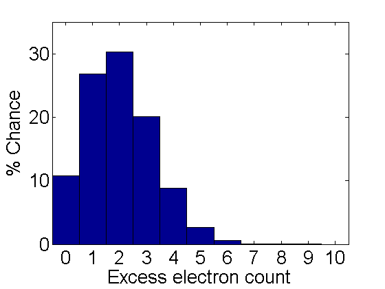
Figure 6. Charge probability.
- Pressure, Temperature, viscosity, and other parameters: All of the properties for the particles are taken from the physical experiment manual. Many of the properties depend on pressure and temperature. The virtual experiment simulates these quantities and displays them on the screen. They change slowly over the day, so be sure to record them when you make your measurements. The pressure is shown in the upper left in kPa. The temperature reading is shown on the upper right as a resistance in a thermistor (temperature sensitive resistor). It is like the photo resistor that we use, but it is sensitive to the temperature. There is a table of resistance and corresponding temperatures in Appendix B in the physical experiment manual. I have made a text file (thermistor.txt) containing the resistance values for your use, but you can also just lookup and interpolate from the table. A plot of the resistance vs. temperature is included below. You will need the temperature to find the viscosity of the air. There is a plot in the physical experiment manual in Appendix A. You may want to print it out for easy use. To get the effective viscosity for the particles you have picked you will use the pressure and a constant
 as well as the radius of the drop. The density of the oil is .
% plot of Resistance vs Temperature
T=10:39;
R=load('thermistor.txt')';
a=polyfit(T,R,4);
plot(T,R,'o',T,polyval(a,T),'linewidth',2);
axis([10 40 1.4 3.3]);
set(gca,'fontsize',20,'xtick',10:3:40,'ytick',1.4:.2:3.3);
xlabel('Temperature');
ylabel('Resistance')
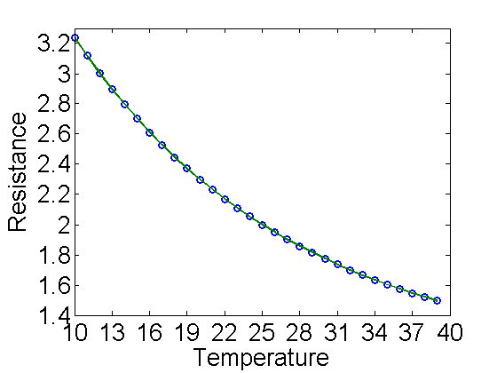
Figure 7. Resistance vs Temperature
Files
- VMOilDrop.zip All files in one zip file.
- VMOilDrop.m (This File).
- VMOilDrop.pdf (pdf version).
- VoltageControl.ino Voltage controller for arduino
- VoltageControlTest.ino Sketch to test the voltage control circuit.
