Biological Application of Tracking

Image data courtesy of Dan Goldman and Vanessa Yip

Contents

Introduction

If you are not familiar with convolution based least-squares fitting please see: Tracking Tutorial.

In many real world tracking problems the objects that need to be tracked are not circular. One approach would be to use least-squares fitting with an idealize shape similar to the object to be tracked. In that case, if we knew the angle of the object, the entire fitting process could not be done with a single convolution. Since in general we do no know the angle, many fits with the idealize shape at different angles would need to be calculated.

Here another approach will be taken. (See also, Long Particle Tracking for an application to rods.) We identify regions of the object which look more like a circle than any other part of the object. Therefore we can fit with a circle at two points on the object and extract the position and angle.

Examine Sample Images

Below is a sample image of an animal that we would like to track.

fignum=1;
dr=dir('*run*.avi'); % get list of movies

% select a frame near the middle of movie
vh=VideoReader(dr(1).name);
raw=read(vh, fix(vh.NumberOfFrames/2));
im=double(raw(:,:,1)); % rgb all same for grayscale movie
simage(im);  % display image in false color
title('Image of an Animal to be Tracked.');
xlabel(sprintf('Figure %d.',fignum)); fignum=fignum+1;

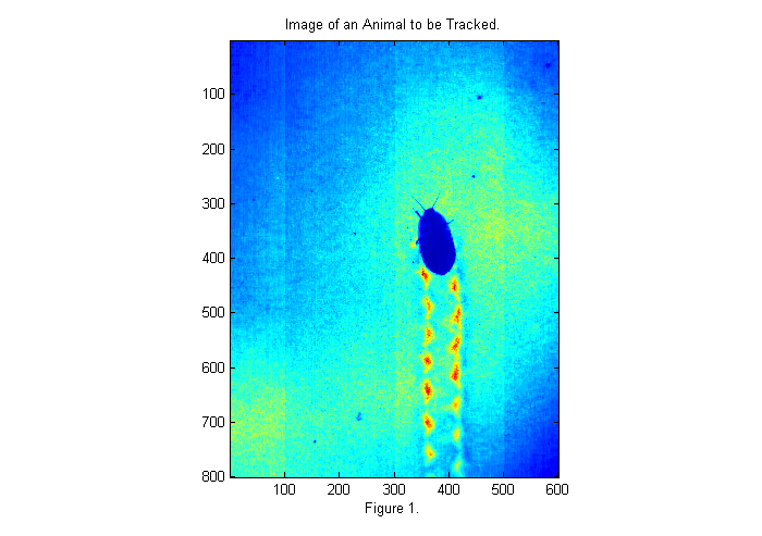
Image Corrections

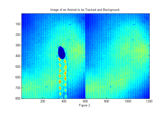
The image above is taken with back-lighting. There are a number of problems that we should fix before tracking. The uneven lighting makes it difficult to track and affects accuracy. To fix this we should take an image of the background (bright background) before we start. It is also a good idea to take an image with the lights covered as well to measure the camera's dark response (dark background). In this case we have neither so will will look to the first image for a bright background as shown below:

raw=read(vh,2);        % read first valid image
bg=double(raw(:,:,1)); % rgb all same for grayscale movie
simage([im bg]);  % display image in false color
title('Image of an Animal to be Tracked and Background.');
xlabel(sprintf('Figure %d.',fignum)); fignum=fignum+1;

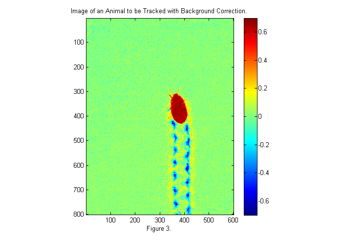
Bright Background Correction

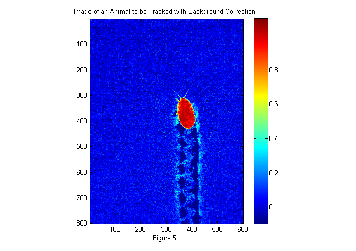
The first image gives a good bright background. The animals antennae are just visible at the bottom of the frame. To use the background we will divide the original image by the background. This will eliminate most of the variations in the lighting. We will also invert the image so that the animal appears bright:

ci=1-im./bg;
simage(ci);  % display image in false color
caxis(.7*[-1 1]);  % set colorscale so that zero is in the middle
colorbar;          % display color bar
title('Image of an Animal to be Tracked with Background Correction.');
xlabel(sprintf('Figure %d.',fignum)); fignum=fignum+1;

Dark Background Correction I

Now the image background is uniform and near zero. Red regions are places where light is blocked (i.e., the animal). Blue regions are places where the image is brighter (i.e., the footprints, where more light is coming through). We would like a normalize image, in which the pixels of the animal are 1 and the background is zero. We are close to that now with the animal ~0.7 and the background at zero. If we had a dark image we could complete the normalization as follows:

$C=\frac{B-I}{B-D},$

where C is the corrected image, I is the original image, B is the bright background, and D is the dark background. If a pixel in the original image is bright then the animal is not there and the corrected image has a value of zero (i.e., I~=B). If a pixel in the original image is dark then the animal is there and the corrected image has a value of 1 (i.e., I~=D). In the previous corrected image we assumed D=0 so that:

$C=\frac{B-I}{B}=1-\frac{I}{B}.$

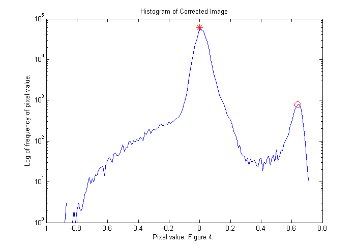
In absence of a true dark image we can use the average pixel value of the dark regions. One way to get it is to look at a histogram of the image:

[nn bb]=hist(ci(:),-1:.01:1);
[~,p1]=max(nn);
nnt=nn;
nnt(bb<.3)=0;
[mx p2]=max(nnt);
dk=bb(p2);

semilogy(bb,nn,bb(p1),nn(p1),'r*',bb(p2),nn(p2),'ro','MarkerSize',10);
ylabel('Log of frequency of pixel value.');
xlabel(['Pixel value. ' sprintf('Figure %d.',fignum)]); fignum=fignum+1;
title('Histogram of Corrected Image');

Dark Background Correction II

The histogram shows the frequency that a given pixel value occurs. For example, the value zero occurs about 64,000 times. This is the largest peak (red *) representing the background. However, there is another peak at about 0.6 (red circle). These are the red pixels that make up the animal. We will find the maximum of the histogram for pixel values greater than 0.3. If we divide the corrected image by this value then the peak will be moved to a pixel value of 1. Also, all of the pixel values less than -.1 are set to -.1 to eliminate the blue spots associated with the foot prints of the animal. This will shift the colorscale so that 1 is red and zero is blue:

ci=ci/dk;
simage(ci);  % display image in false color
caxis([-.1 1.1]);  % set colorscale so that zero is blue
colorbar;          % display color bar
title('Image of an Animal to be Tracked with Background Correction.');
xlabel(sprintf('Figure %d.',fignum)); fignum=fignum+1;

Zoom In I

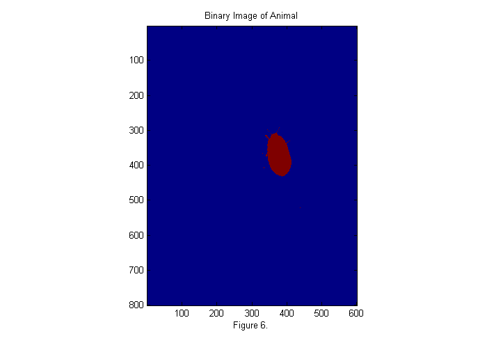
With the background corrected lets zoom in and look at the image. In order to zoom in automatically we need a fast method to locate the animal. One method is to convert the image to binary:

bi=ci>.5;
simage(bi);
title('Binary Image of Animal');
xlabel(sprintf('Figure %d.',fignum)); fignum=fignum+1;

Zoom In II

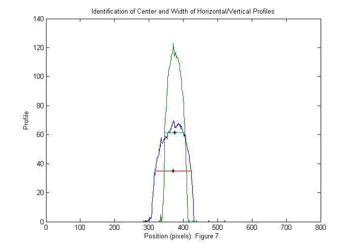
This image is either zero or one. Since we have normalized the image it is easy to set a threshold at 1/2. If we sum this image over x (and y) then we can see a peak where the animal is in y (and x). This also gives us an approximate size in each direction as shown below:

xprof=sum(bi,2);      % sum over horizontal direction
yprof=sum(bi,1);      % sum over vertical direction

% find position of half max of peaks (might use 0.8 of peak to get a better
% estimate of size).
xlim=find(diff(xprof>max(xprof)/2));  % x limits of animal
ylim=find(diff(yprof>max(yprof)/2));  % y limits of animal

cpx=round(mean(xlim));    % crude x position of animal
cpy=round(mean(ylim));    % crude y position of animal

sx=diff(xlim);     % crude x size (smaller than actual animal)
sy=diff(ylim);     % crude y size

plot(1:length(xprof),xprof,...
     1:length(yprof),yprof,...
     xlim,max(xprof)/2*[1 1],...
     ylim,max(yprof)/2*[1 1],...
     cpx,max(xprof)/2,'k*',...
     cpy,max(yprof)/2,'k*');

title('Identification of Center and Width of Horizontal/Vertical Profiles');
ylabel('Profile');
xlabel(['Position (pixels). ' sprintf('Figure %d.',fignum)]); fignum=fignum+1;

Zoom in III

With the crude position and size of the animal determined we can zoom in and take a look. We use twice the size found to be sure we get the whole animal.

im=ci(cpx+(-sx:sx),cpy+(-sy:sy)); % examine small section
im(im<-.1)=-.1;      % remove footprints
simage(im);          % display image in false color
hold on;
th=[0:.01:2*pi 0];
D=23;[~,px,py]=findcircles(double(im>.5),D,.1,1.1*D,6);
plot(py(1)+D/2*sin(th),px(1)+D/2*cos(th),'w');
plot(py(2)+D/2*sin(th),px(2)+D/2*cos(th),'w');
D=50;[~,px,py]=findcircles(im,D,1,1.15*D,5);
plot(py(1)+D/2*sin(th),px(1)+D/2*cos(th),'w');
plot(py(2)+D/2*sin(th),px(2)+D/2*cos(th),'w');
hold off;
caxis([-.1 1.1]);
title('Corrected Image Zoomed in');
xlabel(sprintf('Figure %d.',fignum)); fignum=fignum+1;

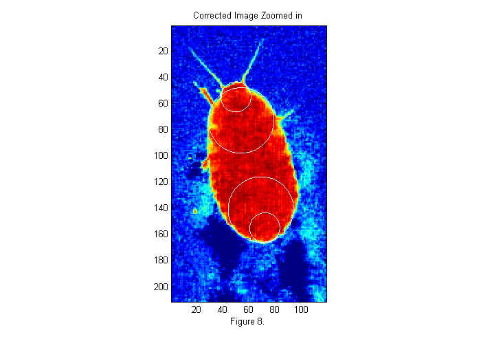
Looking for Circles

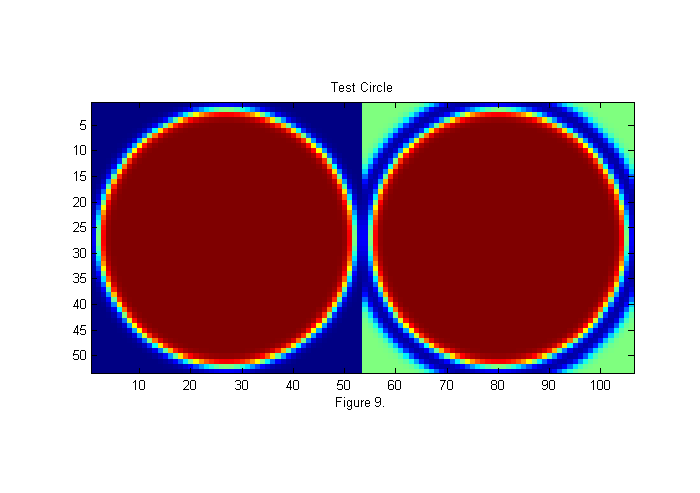
In the expanded image 4 circles have been drawn. These areas of the animal's body look more like a circle than any other parts. Many different circle diameters could be used, but we will focus on the larger circles for now. To see how these circle positions were found we must first create an image of circle to compare with the image. In this case we will use a circle of diameter D=50 pixels. This is the approximate size of the animals abdomen. Here is the code to create the image:

D=50;
[x y]=ndgrid(-fix(D/2)-1:fix(D/2)+1,-fix(D/2)-1:fix(D/2)+1); % ideal particle image grid
r=hypot(x,y);

ip=ipf(r,D,1);  % Create circle

simage([ip ip+.5*(1-ipf(r,1.15*D,1))]);
title('Test Circle');
xlabel(sprintf('Figure %d.',fignum)); fignum=fignum+1;

Least-Squares Fit Function

On the left is a 50 pixel diameter circle. We want to find out what portion of the image most looks like this circle. A common mathematical test for sameness is the Chi-Squared (or Least Squares) fit:

$\chi^2=(X-Y)^2.$

Chi (or chi-squared) is always positive, it is smallest when X is closest to Y, and it is zero if X=Y. We want a function chi which will be smallest at the point in our image which is most like the circle above. Here is a function with those properties:

$\chi^2(\vec{x}_0)=\int [I(\vec{x}) - I_p(\vec{x}-\vec{x}_0)]^2\; d\vec{x},$

where I(x) is our image, Ip is the circle above, and x0 is the test point. The x0 which gives the smallest chi is most like Ip, in this case the circle above. Using convolutions (see: Tracking Tutorial) we can calculate chi-squared as follows:

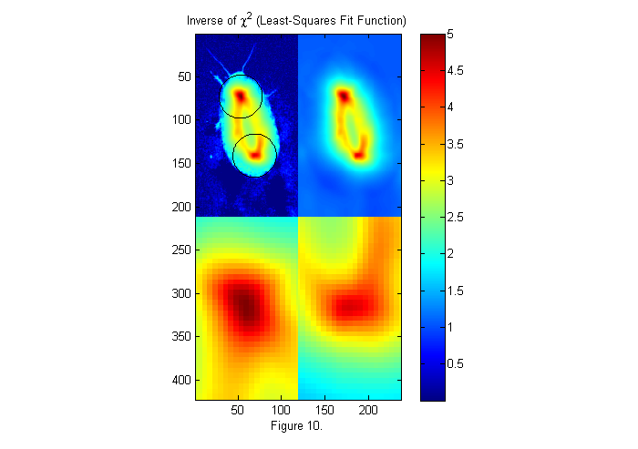
W=ones(size(ip));                   % Weighting factor 1.
ichi=1./chiimg(im,ip,W,[],'same');  % The inverse of the least-squares fit
                                    % function is used since it is easier
                                    % to see peaks than valleys.
[~,px,py]=findpeaks(ichi,1,4,0);   % Find peaks (maxima)
[px ii]=sort(px(1:2));    % Head first (see below)
py=py(ii);

% create zoomed images
lx=-fix(sx/6)-1:fix(sx/6)+1;
ly=-fix(sy/6)-1:fix(sy/6)+1;
llx=(-sx:sx)/6;
lly=(-sy:sy)/6;

zi1=interp2(ly,lx,ichi(px(1)+lx,py(1)+ly),lly,llx','nearest');
zi2=interp2(ly,lx,ichi(px(2)+lx,py(2)+ly),lly,llx','nearest');

simage([ichi.*(ichi>2)+2*im.*(ichi<2) ichi; zi1 zi2]);
caxis([0 max(ichi(:))]);
hold on;
plot(py(1)+D/2*sin(th),px(1)+D/2*cos(th),'k');
plot(py(2)+D/2*sin(th),px(2)+D/2*cos(th),'k');
hold off;
title('Inverse of \chi^2 (Least-Squares Fit Function)');
colorbar;
xlabel(sprintf('Figure %d.',fignum)); fignum=fignum+1;

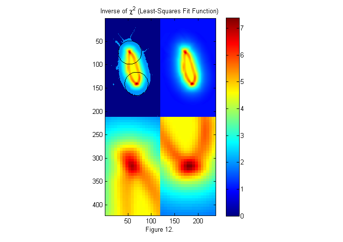
Weighted Fit Function

The image on the upper right is 1/chi-squared as a function x0. For convenience we look at 1/chi instead of chi so that the best fit is a peak. On the upper left, the image of the animal is superimposed along with the best circles. In the lower images, the two peaks (maxima of 1/chi or minima of chi) are expanded. The test image shown on the left of figure 9 is square. Chi-squared tests the whole square so we are really looking for a circle of intensity one in a square of square of intensity zero. If we made the square bigger we would get a different fit. To incorporate this idea into chi directly we use a weighted chi-squared:

$\chi^2(\vec{x}_0)=\int W(\vec{x}-\vec{x}_0)[I(\vec{x}) - I_p(\vec{x}-\vec{x}_0)]^2\; d\vec{x},$

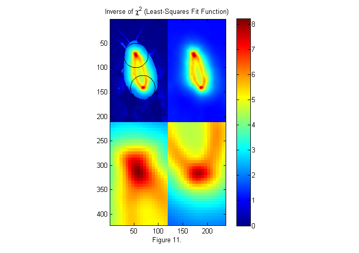
where W(x) is the weight function. In the chi shown in figure 10 the weight is set to 1 so the whole test image is used. Often more robust and accurate results are obtained using a circular weighting function. For example the right side of figure 9 represents a weighted test image, in which the green portions are set to zero and therefore ignored. We do this by using a weight function which is a circle slightly larger than our test circle. In this case, 15% larger. This will help make the peaks sharper and taller, as seen below.

W=ipf(r,1.15*D,1);                  % Circular weighting factor 15% larger
ichi=1./chiimg(im,ip,W,[],'same');  % The inverse of the least-squares fit
                                    % function is used since it is easier
                                    % to see peaks than valleys.
[~,px,py]=findpeaks(ichi,1,4,0);   % Find peaks (maxima)
[px ii]=sort(px(1:2));    % Head first (see below)
py=py(ii);

% create zoomed images
zi1=interp2(ly,lx,ichi(px(1)+lx,py(1)+ly),lly,llx','nearest');
zi2=interp2(ly,lx,ichi(px(2)+lx,py(2)+ly),lly,llx','nearest');

simage([ichi.*(ichi>2)+2*im.*(ichi<2) ichi; zi1 zi2]);
caxis([0 max(ichi(:))]);
hold on;
plot(py(1)+D/2*sin(th),px(1)+D/2*cos(th),'k');
plot(py(2)+D/2*sin(th),px(2)+D/2*cos(th),'k');
hold off;
title('Inverse of \chi^2 (Least-Squares Fit Function)');
colorbar;
xlabel(sprintf('Figure %d.',fignum)); fignum=fignum+1;

Fitting to a Binary Image

In the frame shown above, the background corrections worked well. Therefore, fitting to the full (real) image works well. However, in some cases the correction may not as good. For example near the edges of an image the dark response is often not as good. If the animal image is not uniform, we can fit to a binary image like we used for the crude subject locater above. In this way, the image is always either 0 or 1, but the edges may be less accurate. Typically, the full image is used unless there are regions were the subject is not uniform enough for a good fit. Below is the weighted fit function using a binary image.

% use binary image
bi=ci>.5;
im=double(bi(cpx+(-sx:sx),cpy+(-sy:sy))); % examine small section

W=ipf(r,1.15*D,1);                  % Circular weighting factor 15% larger
ichi=1./chiimg(im,ip,W,[],'same');  % The inverse of the least-squares fit
                                    % function is used since it is easier
                                    % to see peaks than valleys.
[~,px,py]=findpeaks(ichi,1,4,0);   % Find peaks (maxima)
[px ii]=sort(px(1:2));    % Head first (see below)
py=py(ii);

% create zoomed images
zi1=interp2(ly,lx,ichi(px(1)+lx,py(1)+ly),lly,llx','nearest');
zi2=interp2(ly,lx,ichi(px(2)+lx,py(2)+ly),lly,llx','nearest');

simage([ichi.*(ichi>2)+2*im.*(ichi<2) ichi; zi1 zi2]);
caxis([0 max(ichi(:))]);
hold on;
plot(py(1)+D/2*sin(th),px(1)+D/2*cos(th),'k');
plot(py(2)+D/2*sin(th),px(2)+D/2*cos(th),'k');
hold off;
title('Inverse of \chi^2 (Least-Squares Fit Function)');
colorbar;
xlabel(sprintf('Figure %d.',fignum)); fignum=fignum+1;

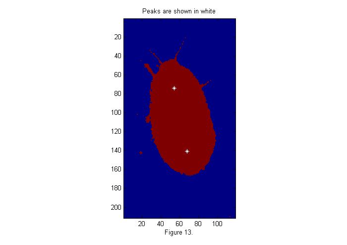
Extract Peak Positions

For any of the fit functions above we need to extract the peak positions. The findpeaks function finds all peaks, which are greater than a threshold, in this case 6 works well.

MinSep=0;        % minimum separation between peaks
Cutoff=6;        % minimum peak intensity
[Np spx spy]=findpeaks(ichi,1,Cutoff,MinSep);

simage(im);
hold on;
plot(spy,spx,'w*');
hold off;
title('Peaks are shown in white');
xlabel(sprintf('Figure %d.',fignum)); fignum=fignum+1;

Putting it All Together

The m-file trackfile.m is a simple script which combines all of the parts above into a single script to track a complete file BN6_0_1_2_run_soft_xvid.avi. The results are stored as trackfile_bi_BN6_0_1_2_run_soft_xvid.mat and trackfile_ci_BN6_0_1_2_run_soft_xvid.mat.

trbifn='trackfile_bi_BN6_0_1_2_run_soft_xvid.mat';
trcifn='trackfile_ci_BN6_0_1_2_run_soft_xvid.mat';

if(~exist(trbifn,'file'))  % check for trackfiles
  clear all;           % Start from scratch
  clear all
  UseBinImg=true;      % use binary image
  trackfile;
end
if(~exist(trcifn,'file')) % check for trackfiles
  clear all;           % Start from scratch
  UseBinImg=False;     % use full image
  trackfile;
end

load(trcifn);  % Load full image results
pxc=px;
pyc=py;
ppxc=ppx;
ppyc=ppy;

load(trbifn);  % Load binary image results

plot(px');
title('Animal Position vs. Time');
ylabel('Vertical Position (pixels)');
xlabel(['Time (frame number). ' sprintf('Figure %d.',fignum)]); fignum=fignum+1;
text(310,px(1,300),'\leftarrow Tail','HorizontalAlignment','left');
text(300,px(2,300),'Head \rightarrow','HorizontalAlignment','right');

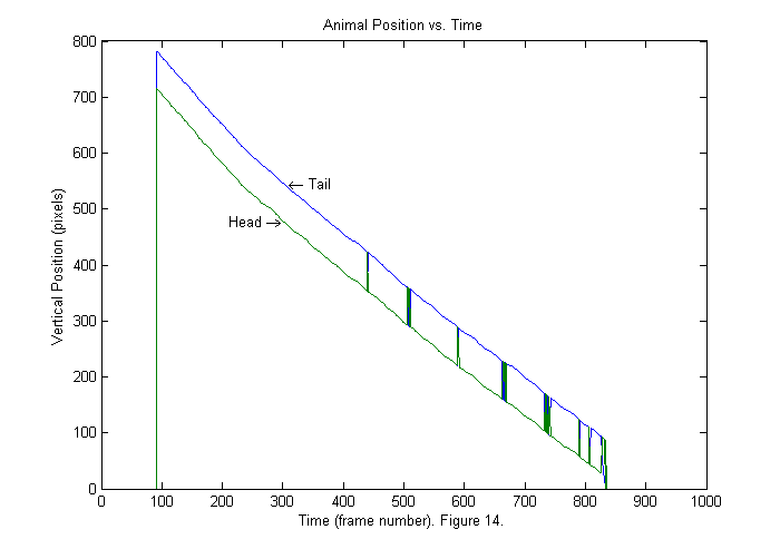
Results I (Sorting Heads from Tails)

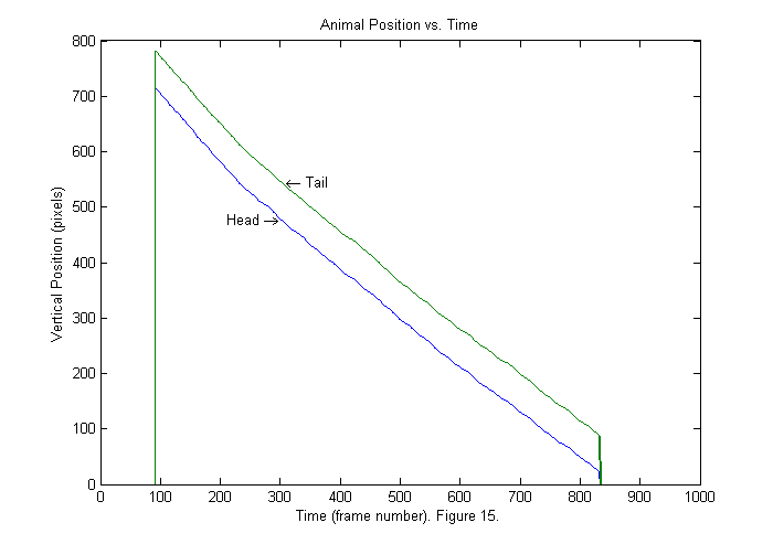
The vertical positions of head and tail as a function of frame number are shown above. The order of the points found is based on the size of the peak in the fit function so sometimes the tail is blue indicating that it is first and sometimes the tail is green indicating that it is second. In this example we can determine which is which by noticing that the head is always ahead of the tail in the vertical directions. In other cases, we may need to use a more sophisticated method. For example, if the animal is moving forward then the velocity direction points in the direction of the head. Also the head can not move a distance of the whole body in one frame. Therefore the head position in the frame n+1 should be near the head position in frame n. Below is a repeat of the same plot sorted by vertical position.

[spx ii]=sort(px); % Sort by vertical position.
spy=zeros(size(spx));
for nf=1:length(ii)    % Sort horizontal position using vertical index ii.
  spy(:,nf)=py(ii(:,nf),nf);
end

plot(spx');
title('Animal Position vs. Time');
ylabel('Vertical Position (pixels)');
xlabel(['Time (frame number). ' sprintf('Figure %d.',fignum)]); fignum=fignum+1;
text(310,px(1,300),'\leftarrow Tail','HorizontalAlignment','left');
text(300,px(2,300),'Head \rightarrow','HorizontalAlignment','right');

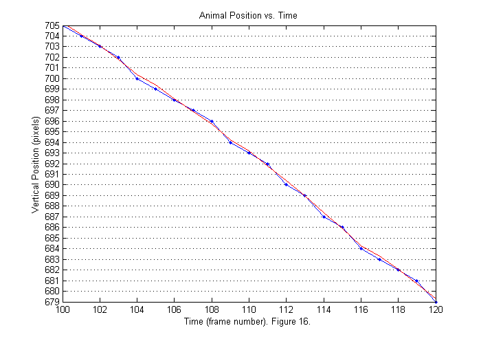
Results II (Interpolation)

Now the head is in the first position all of the time. The tracking script tries to detect when the whole animal first enters the frame. In this case that occurs around frame 90. The animal leaves around frame 830. If we zoom in (see below) we will see that the positions that findpeaks locates are all integers (blue). We can produce a smoother trajectory (red) by using interpolation around the fit function peak. Interpolation is included in the trackfile script, but is not explained in detail. Later an update to these notes will be added on interpolation and other subpixel methods. To see how to get the interpolated results examine the lines below:

[sppx ii]=sort(px+ppx); % Sort by vertical position.
                        % px (py) is list of pixel accurate positions. ppx
                        % (ppy) is a correction to px (py).  So px+ppx is
                        % sub-pixel accurate.
sppy=zeros(size(spx));
for nf=1:length(ii)    % Sort horizontal position using vertical index ii.
  sppy(:,nf)=py(ii(:,nf),nf)+ppy(ii(:,nf),nf);
end

plot(1:Nf,spx','.-',1:Nf,sppx');
axis([100 120 spx(1,120) spx(1,100)])
set(gca,'ygrid','on','Ytick',spx(1,120):spx(1,100))
title('Animal Position vs. Time');
ylabel('Vertical Position (pixels)');
xlabel(['Time (frame number). ' sprintf('Figure %d.',fignum)]); fignum=fignum+1;

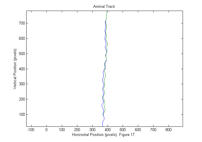
Results III (Animal Track)

We can now show the animal track. The head track is blue and the tail track is green.

good=find(Npf==2);  % find good frames
plot(sppy(:,good)',sppx(:,good)');
axis('equal');
title('Animal Track');
ylabel('Vertical Position (pixels)');
xlabel(['Horizontal Position (pixels). ' sprintf('Figure %d.',fignum)]); fignum=fignum+1;

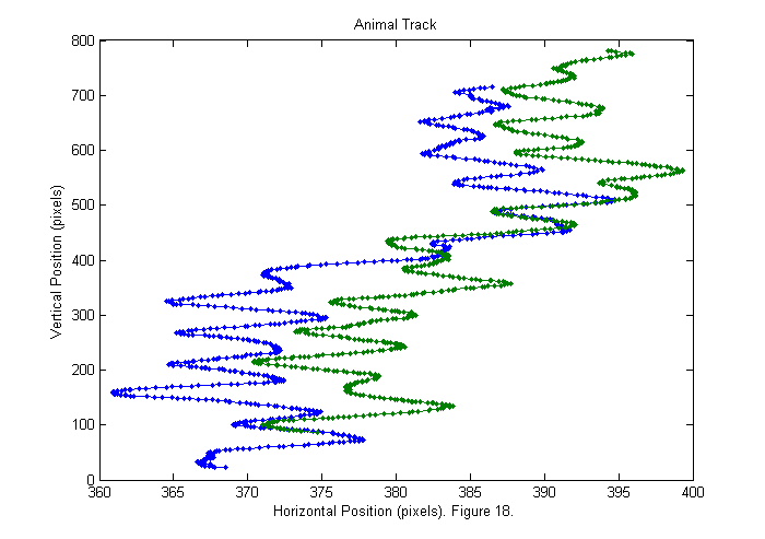
Results IV (Animal Track)

If we expand the horizontal axis we can see that the animal wobbles from side to side.

good=find(Npf==2);  % find good frames
plot(sppy(:,good)',sppx(:,good)','.-');
title('Animal Track');
ylabel('Vertical Position (pixels)');
xlabel(['Horizontal Position (pixels). ' sprintf('Figure %d.',fignum)]); fignum=fignum+1;

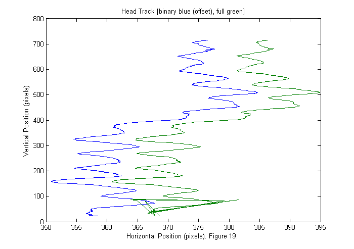
Results V (Binary vs. Full)

Below the head track is shown for both the binary image (blue) and the full image (green). The binary is shifted by 10 pixels for clarity. Generally the full appears smoother, which is typically a sign of higher accuracy. However, the background correction is not good enough near the top edge of the image, and the tracking fails to find the head properly in the last 20 frames. With the current data we can not tell which is more accurate. To do that we need to track something with a know position, such as an object attached to a micrometer. Therefore for this data set the binary is probably best as it gives a works over a larger range.

[sppxc ii]=sort(pxc+ppxc); % Sort by vertical position.
                           % px (py) is list of pixel accurate positions. ppx
                           % (ppy) is a correction to px (py).  So px+ppx is
                           % sub-pixel accurate.
sppyc=zeros(size(sppxc));
for nf=1:length(ii)    % Sort horizontal position using vertical index ii.
  sppyc(:,nf)=pyc(ii(:,nf),nf)+ppyc(ii(:,nf),nf);
end

plot(sppy(1,good)'-10,sppx(1,good)',sppyc(1,good)',sppxc(1,good)');
title('Head Track [binary blue (offset), full green]');
ylabel('Vertical Position (pixels)');
xlabel(['Horizontal Position (pixels). ' sprintf('Figure %d.',fignum)]); fignum=fignum+1;

m-files

Published with MATLAB® 7.14