Particle Tracking

A tutorial using convolution based least-squares fitting.

Contents

Theory

Idealize Particle Function

We assume that the image to be tracked is of the form:

$I_c(\vec{x})=\sum_{n=1}^{N} I_p(\vec{x}-\vec{x}_n(t);D,...),\;\;\;\;\;\;[1]$

where N is the number of particles and

$I_p(\vec{x};D,...)$

is a function describing the shape of an idealized particle centered at the origin. The ideal particle function may depend on the diameter of the particle or other properties of the particle or imaging system.

For this demonstration we will use:

$I_p(\vec{x};D,w)=[1-tanh(\frac{|\vec{x}|-D/2}{w})]/2.$

This function is implemented in ipf.m. It smoothly varies between 1 inside the particle, 1/2 on the particle boundary and 0 outside of the particle. The parameter w determines how sharply the function changes (76% change over a range of +/-w). In principle, w can be related to the focus of the imaging system through the point-spread function. Smaller values of w correspond to sharper focus. A value of 1/2 represents a good sharp focus. The functional form is shown here:

Functional Form of Ideal Particle

x=-10:.1:10;
D=12;          % Diameter
w=1.3;         % Width
h=figure(2); set(h,'Position',[100 100 400 300],'Color',[1 1 1]);
plot(x,ipf(x,D,w),D/2*[1 1],[1/(1+exp(2)) 1/(1+exp(-2))],D/2*[1 1]-w,[0 1],D/2*[1 1]+w,[0 1],(w*[-1 1])+D/2,1/(1+exp(2))*[1 1],(w*[-1 1])+D/2,1/(1+exp(-2))*[1 1])
text(6,.9,'{\it 2w}','HorizontalAlignment','center');
text(6.5,.5,'76%');
xlabel('Position (Figure 1)');
ylabel('Intensity');

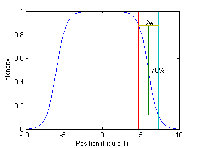
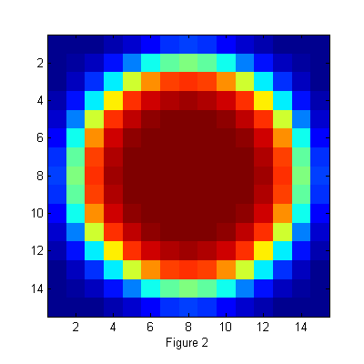
Image of Ideal Particle

D=12;          % Diameter
w=1.3;         % Width
ss=2*fix(D/2+4*w/2)-1;          % size of ideal particle image
os=(ss-1)/2;                    % (size-1)/2 of ideal particle image
[xx yy]=ndgrid(-os:os,-os:os);  % ideal particle image grid
r=hypot(xx,yy);                 % radial coordinate
h=figure(2); set(h,'Position',[100 100 400 400],'Color',[1 1 1]);
simage(ipf(r,D,w));
xlabel('Figure 2');

Least-Squares Fit Function: chi-squared

We can find the most likely position of a particle using least-squares-fitting. First we define chi-squared:

$\chi^2(\vec{x}_0;D,w)=\int W(\vec{x}-\vec{x}_0)[I(\vec{x}) - I_p(\vec{x}-\vec{x}_0;D,w)]^2\; d\vec{x},\;\;\;\;\;[2]$

where W(x-x0) is a weight function. The domain of integration is over the area of the experimental image I. However the domain of x0 is larger. In general, if the size of the image is Lx by Ly and the size of Ip is sx by sy then the range of integration is [0 Lx] and [0 Ly] but the range of x0 is [-sx Lx+sx] and [-sy Ly+sy].

When x0 is at the position of a particle then chi-squared will be minimum. Therefore if we minimize chi-squared over x0 then we can find the particle's position. In fact, there will be a minimum in chi-squared at the position of each particle. If the image is exactly that of eq. [1] then chi-squared will be zero for each x0=xn.

So the process of finding the particles is equivalent to finding all of the minima of chi-squared. We can use convolution to do this easily. Expanding eq. [2]:

$\chi^2(\vec{x}_0;D,w)=\int W(\vec{x}-\vec{x}_0)[I(\vec{x})^2 - 2I(\vec{x})I_p(\vec{x}- \vec{x}_0;D,w)+I_p(\vec{x}-\vec{x}_0;D,w)^2]\; d\vec{x},$

$\chi^2(\vec{x}_0;D,w)=I^2 \otimes W - 2I \otimes (W I_p) + <W I_p^2>,\;\;\;\;\;[3]$

where

$f\otimes g = [f\otimes g](\vec{x}_0)=\int f(\vec{x})g(\vec{x}-\vec{x}_0)\;d\vec{x},\;\;\;\;\;[4]$

and

$<f>=1 \otimes f,$

which is not simply a constant, but a function of x0 since domain of integration is over the image only. If W or Ip are not symmetric then care must be take to evaluate eq [4] (which is actually a cross-correlation) using convolution, defined as,

$f*g = [f*g](\vec{x}_0)=\int f(\vec{x})g(\vec{x}_0-\vec{x})\;d\vec{x}=f(\vec{x}) \otimes g(-\vec{x}).$

Direct cross-correlation

Several choices are possible for the weight function. If

$W=1;\;\;\;\;\; \chi^2(\vec{x}_0;D,w)= \int I^2\;d\vec{x} - 2I \otimes I_p + <I_p^2>,$

In this case, the first term does not depend on x0 and the last term only depends on the x0 near the edge of the image. Thus

$I \otimes I_p$

will be maximum for x0 at the particle positions. The fact that the cross-correlation is maximum near particle centers is the starting point for many particle tracking techniques. From the previous discussion, we can see the basis for this ansatz is the minimization of chi-squared. This technique works well for images in which the particles are well separated and have good signal-to-noise. This is because the weight function is very broad making the fit sensitive to the fact that the ideal particle image has zeros all around it in contrast to the real image in which other particles are nearby. This choice of W also produces a broad peak to maximize making it sensitive to noise.

Full chi-squared minimization

We find that a compact weight function produces much better results. We typically use:

$W=I_p;\;\;\;\;\; \chi^2(\vec{x}_0;D,w)=I^2 \otimes I_p - 2I \otimes I_p^2 + <I_p^3>.$

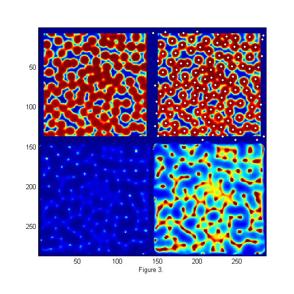
The first term of chi-squared shows that only the area of size Ip around each point x0 is important. The last term is a constant except near the edges of the image. Near the edge it and all of the terms get smaller due to the fact that there is less and less overlap between the experimental image I and the ideal particle image Ip. So to normalize this effect at the boundary we divide through by the last term and define a new chi-squared:

$\chi^2(\vec{x}_0;D,w)=\frac{I^2 \otimes I_p - 2I \otimes I_p^2}{<I_p^3>}+1.\;\;\;\;\;[5]$

Equation [5] is implemented in chiimg.m, which can also calculate a normalized version of eq. [3]:

$\chi^2(\vec{x}_0;D,w)=\frac{I^2 \otimes W - 2I \otimes WI_p}{<WI_p^2>}+1.$

This normalized chi-squared is still minimized at the positions of particles, and can be used to find particles which have centers outside of the image. Here is an example:

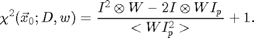
Image of particles in a dense state and Corresponding Chi-Squared

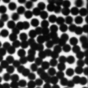
raw=imread('test.bmp');  % load image
[Nx Ny]=size(raw);       % image size

hi=250;  % hi and lo values come the image histogram
lo=10;   % hi/lo=typical pixel value outside/inside
ri=(hi-double(raw))/(hi-lo);  % normalize image

D=12;          % Diameter
w=1.3;         % Width
ss=2*fix(D/2+4*w/2)-1;          % size of ideal particle image
os=(ss-1)/2;                    % (size-1)/2 of ideal particle image
[xx yy]=ndgrid(-os:os,-os:os);  % ideal particle image grid
r=hypot(xx,yy);                 % radial coordinate

Cutoff=5;      % minimum peak intensity
MinSep=5;      % minimum separation between peaks
[Np px py]=findpeaks(1./chiimg(ri,ipf(r,D,w)),1,Cutoff,MinSep);  % find maxima

h=figure(2); set(h,'Position',[100 100 600 600],'Color',[1 1 1]);
simage([100*zerofill(ri,2*os,2*os) 100*zerofill(ri,2*os,2*os); 1./chiimg(ri,ipf(r,D,w)) 8*1./chiimg(ri,ipf(r,D,w))]); caxis([0 100])
hold on;
plot(py+2*os+Ny,px,'w.');
hold off;
xlabel('Figure 3.');

Finding Particle Centers

An image of monodisperse particles at approximately 0.8 area fraction is shown the upper left of fig. 3. The image is relatively low resolution, with good signal to noise. The focus is not very sharp. This image represents a typical image to be tracked. The raw image is taken using back lighting so that particle appear dark. The displayed image has been normalize using the bright and dark peaks from the histogram of the image so that intensities are approximately 1 inside and 0 outside of the particles. In the lower left, chi-squared from eq. [5] is shown. Ip is from fig. 2. For visualization the inverse of chi-squared is shown so that particle centers appear as bright peaks. In the lower right image 1/chi-squared is shown again 8 times brighter to allow visualization of the smaller peaks. A function findpeaks.m is used to extract all of the peaks (maxima) in 1/chi-squared. It finds all pixels which are larger than their 8 nearest neighbors, have intensities greater than a 'Cutoff', and are separated from all other peaks by at least 'MinSep' pixels. The results are 122 peaks found. The white dots in the upper right image shows the particles found. We are able to find all of the particles and partial particles even in this dense state with relatively low resolution of 12 pixels/particle and poor focus. This gives particle centers to approximately one pixel accuracy.

Sub-pixel accuracy using least-squares fitting

We can also use least-squares fitting to determine the particle centers to sub-pixel accuracy. To do this we will look a modified chi-squared:

$\chi^2(\vec{x}_n;D,w)=\int [I(\vec{x}) - I_c(\vec{x},\vec{x}_n)]^2\; d\vec{x},\;\;\;\;\;[6]$

where

$I_c(\vec{x},\vec{x}_n)=\sum_n W_n(\vec{x})I_p(\vec{x}-\vec{x}_n;D,w),$

and Wn is a function which is one inside the Voronoi volume of particle n and zero outside. Wn takes care of particles which are overlapping. We implement Ic using pgrid.m and ipf.m. Here is an example calculating Ic and chi-squared.

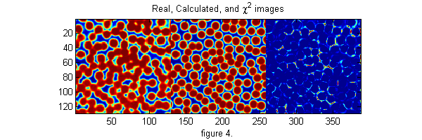
[cxy over]=pgrid(px-os,py-os,Nx,Ny,[1 Nx 1 Ny],Np,2*os+3,0); % create local grid centered on each particle and overlap matrix
ci=ipf(cxy,D,w);  % create calculated image

di=ci-ri;                             % Calculate difference image
h=figure(2); set(h,'Position',[100 100 600 200],'Color',[1 1 1]);
simage([ri ci 4*di.^2]); caxis([0 1])   % Show the real, calculated, and chi-squared image
title('Real, Calculated, and \chi^2 images')
xlabel('figure 4.')

chi2=sum(di(:).^2);                   % Calculate Chi-Squared
fprintf('Chi-Squared=%f\n',chi2);

chi2o=chi2;di0=di;  % save for later

Chi-Squared=228.162463

Minimizing chi-squared

To find the centers of the particles we want to minimize the average of the square of the third image above, which is equivalent to solving,

$\frac{\partial\chi^2(\vec{x}^*_n;D,w)}{\partial\vec{x}^*_n}=0,\;\;\;\;\;$

for the xn*. Since we have a good pixel accurate guess we can solve using Newton's method. One Newton's step is implemented in cidp2.m. This function returns the change in xn needed to bring the equations closer to solution. By calling it multiple times the solution is determined. Here is an example:

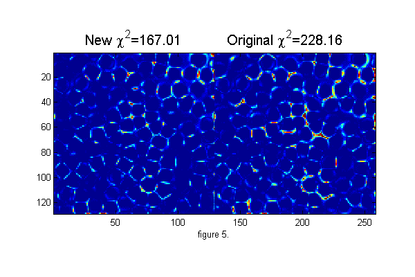
maxnr=5;       % maximum number of calls to Newton solver.
mindelchi2=1;  % minimum change in chi2 before stopping

nr=0;
delchi2=1e99;
while((abs(delchi2)>mindelchi2) && (nr<maxnr))
  [dpx dpy]=cidp2(cxy,over,di,Np,D,w);  %
  px=px+dpx;
  py=py+dpy;
  [cxy over]=pgrid(px-os,py-os,Nx,Ny,[1 Nx 1 Ny],Np,2*os+3,0); % create local grid centered on each particle and overlap matrix
  ci=ipf(cxy,D,w);  % create calculated image
  di=(ci-ri);
  delchi2=chi2-sum(di(:).^2); % Calculate change in Chi-Squared
  chi2=chi2-delchi2;          % Calculate Chi-Squared
  fprintf('.');
  nr=nr+1;
end
fprintf('\n');
chi2=sum(di(:).^2);                     % Calculate Chi-Squared
fprintf('Chi-Squared=%f\n',chi2);

h=figure(2); set(h,'Position',[100 100 600 400],'Color',[1 1 1]);
simage([di.^2 di0.^2]); caxis([0 .25]); % Show the chi-squared images
title(sprintf('New \\chi^2=%6.2f           Original \\chi^2=%6.2f',chi2,chi2o),'fontsize',15)
xlabel('figure 5.')

...
Chi-Squared=167.009367

Finding D and w

The image above shows the improvement in chi-squared. The user inputs to this technique are the diameter and width parameter for the ideal particle image. From a good guess we can calculate better values by minimizing chi-squared over D and w. That is, finding D* and w* from these equations:

$\frac{\partial\chi^2(\vec{x}_0;D^*,w^*)}{\partial D^*}=0;\;\;\;\;\; \frac{\partial\chi^2(\vec{x}_0;D^*,w^*)}{\partial w^*}=0$

We use Newton's method to solve these equations. One Newton's step is implemented in cidDw.m. This function returns the change in D and w needed to bring the equations closer to solution. By calling it multiple times the solution is determined. Here is an example:

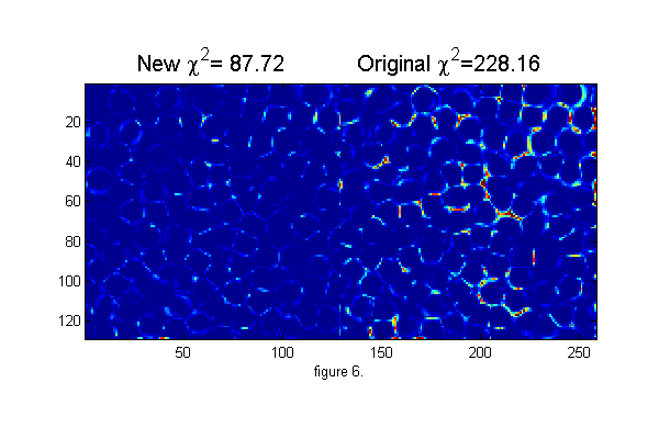
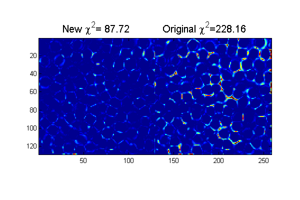
% start over with pixel accurate positions
Cutoff=5;      % minimum peak intensity
MinSep=5;      % minimum separation between peaks
[Np px py]=findpeaks(1./chiimg(ri,ipf(r,D,w)),1,Cutoff,MinSep);  % find maxima

[cxy over]=pgrid(px-os,py-os,Nx,Ny,[1 Nx 1 Ny],Np,2*os+3,0);  % create local x y grid
ci=ipf(cxy,D,w);  % create calculated image

di=ci-ri;  %

maxDwnr=10;       % maximum number of calls to cidDw Newton solver.
mindelD=.0001;    % minimum change in D before stopping

nr=0;
delD=1;
while((abs(delD)>mindelD) && nr<maxDwnr)
  [delD delw]=cidDw(abs(cxy),di,D,w);
  D=D+delD;
  w=w+delw;
  ci=ipf(abs(cxy),D,w);
  di=(ci-ri);
  fprintf('.');
  nr=nr+1;
end
fprintf('\n');
chi2=sum(di(:).^2);
fprintf('Chi-Squared=%f\n',chi2);

% Repeat position minimization

nr=0;
delchi2=1e99;
while((abs(delchi2)>mindelchi2) && (nr<maxnr))
  [dpx dpy]=cidp2(cxy,over,di,Np,D,w);  %
  px=px+dpx;
  py=py+dpy;
  [cxy over]=pgrid(px-os,py-os,Nx,Ny,[1 Nx 1 Ny],Np,2*os+3,0); % create local grid centered on each particle and overlap matrix
  ci=ipf(cxy,D,w);  % create calculated image
  di=(ci-ri);
  delchi2=chi2-sum(di(:).^2); % Calculate change in Chi-Squared
  chi2=chi2-delchi2;          % Calculate Chi-Squared
  fprintf('.');
  nr=nr+1;
end
fprintf('\n');
chi2=sum(di(:).^2);                     % Calculate Chi-Squared
fprintf('Chi-Squared=%f\n',chi2);

h=figure(2); set(h,'Position',[100 100 600 400],'Color',[1 1 1]);
simage([di.^2 di0.^2]); caxis([0 .25]); % Show the chi-squared images
title(sprintf('New \\chi^2=%6.2f           Original \\chi^2=%6.2f',chi2,chi2o),'fontsize',15)
xlabel('figure 6.')

.....
Chi-Squared=154.184859
...
Chi-Squared=87.717465

Putting it all together

Below is and example of a code to track one frame from start to finish. It is also available separately as trackframe.m

clear('all');
% <trackframe.m> Mark D. Shattuck 3/29/2008
% Particle tracking demonstration

% User Inputs
D=12;          % Initial Diameter Guess
w=1.3;         % Initial Width Guess
Cutoff=5;      % minimum peak intensity
MinSep=5;      % minimum separation between peaks

hi=250;  % hi and lo values come the image histogram
lo=10;   % hi/lo=typical pixel value outside/inside

maxDwnr=10;       % maximum number of calls to cidDw Newton solver.
mindelD=.0001;    % minimum change in D before stopping

maxnr=5;       % maximum number of calls to cidp2 Newton solver.
mindelchi2=1;  % minimum change in chi2 before stopping

% setup for ideal particle

ss=2*fix(D/2+4*w/2)-1;          % size of ideal particle image
os=(ss-1)/2;                    % (size-1)/2 of ideal particle image
[xx yy]=ndgrid(-os:os,-os:os);  % ideal particle image grid
r=hypot(xx,yy);                 % radial coordinate

raw=imread('test.bmp');  % load image
[Nx Ny]=size(raw);       % image size

ri=(hi-double(raw))/(hi-lo);  % normalize image

% find pixel accurate centers using chi-squared

[Np px py]=findpeaks(1./chiimg(ri,ipf(r,D,w)),1,Cutoff,MinSep);  % find maxima

% Minimizing chi-squared for sub-pixel accuracy

[cxy over]=pgrid(px-os,py-os,Nx,Ny,[1 Nx 1 Ny],Np,2*os+3,0); % create local grid centered on each particle and overlap matrix
ci=ipf(cxy,D,w);  % create calculated image

di=ci-ri;                             % Calculate difference image
chi2=sum(di(:).^2);                   % Calculate Chi-Squared
fprintf('Chi-Squared=%f\n',chi2);

chi2o=chi2;di0=di;  % save for later

% find best D and w
nr=0;
delD=1e99;
while((abs(delD)>mindelD) && (nr<maxDwnr))
  [delD delw]=cidDw(abs(cxy),di,D,w);
  D=D+delD;
  w=w+delw;
  ci=ipf(abs(cxy),D,w);
  di=(ci-ri);
  fprintf('.');
  nr=nr+1;
end
fprintf('\n');
chi2=sum(di(:).^2);
fprintf('Chi-Squared=%f\n',chi2);

% Find best positions
nr=0;
delchi2=1e99;
while((abs(delchi2)>mindelchi2) && (nr<maxnr))
  [dpx dpy]=cidp2(cxy,over,di,Np,D,w);  %
  px=px+dpx;
  py=py+dpy;
  [cxy over]=pgrid(px-os,py-os,Nx,Ny,[1 Nx 1 Ny],Np,2*os+3,0); % create local grid centered on each particle and overlap matrix
  ci=ipf(cxy,D,w);  % create calculated image
  di=(ci-ri);
  delchi2=chi2-sum(di(:).^2); % Calculate change in Chi-Squared
  chi2=chi2-delchi2;          % Calculate Chi-Squared
  fprintf('.');
  nr=nr+1;
end
fprintf('\n');
chi2=sum(di(:).^2);                     % Calculate Chi-Squared
fprintf('Chi-Squared=%f\n',chi2);

h=figure(2); set(h,'Position',[100 100 600 400],'Color',[1 1 1]);
simage([di.^2 di0.^2]); caxis([0 .25]); % Show the chi-squared images
title(sprintf('New \\chi^2=%6.2f           Original \\chi^2=%6.2f',chi2,chi2o),'fontsize',15)

Chi-Squared=228.162463
.....
Chi-Squared=154.184859
...
Chi-Squared=87.717465

Discussion of Accuracy

The positions in the example above have an accuracy of about 1/10 of a
pixel.  With a little higher resolution ~ 20 pixels/particle images and
better focus it is easy to achieve 1/100 of a pixel resolution.  With
our best imaging using ~ 60 pixels/particle we can achieve 1/1000 of a
pixel accuracy which gives us 50 nm resolution on 3.175 mm particle at
60,000 frames per second.

m-files

Image files

Published with MATLAB® 7.14