Molecular Dynamics Simulation Laboratory
Part I: Distributions and Equation of State.
- [ MDLabI.pdf ] pdf version.
- [ MDLabI.php ] html version.
Contents
Introduction
A Molecular Dynamics (MD) simulation is a computer simulation of Newton's Laws for a collection of particles. For a brief introduction to molecular dynamics please see: An introduction to molecular dynamics in Matlab. In part I of this lab, we will focus on systems with fixed Number, Volume (area), and Energy  . We say these systems are in the microcanonical ensemble. The matlab code we will uses is a script mdNVE000.m, which requires one helper file plotNCirc.m to function.
Matlab has two main ways to store programs---scripts and functions. A script is just a list of commands stored in a file that are run sequentially. A function takes input variables and returns variables, but anything inside is hidden. We will use a script so that we have access to all of the internal variables. You can freely edit mdNVE000.m, but it is setup so that it is not necessary. The code has comments on most lines. Comments are any text after a % sign. Comments can not be nested.
Exercise I
Running the code:
- Getting the code: You need to download 2 files by (right-clicking -> save link as... on PC) or (Control-clicking -> save link as... on MAC) mdNVE000.m and plotNCirc.m or by downloading and unzipping MDLabI.zip. Download and put both files in a new directory or unzip to a new directory.
- Open matlab and change to the directory where you put mdNVE000.m and plotNCirc.m.
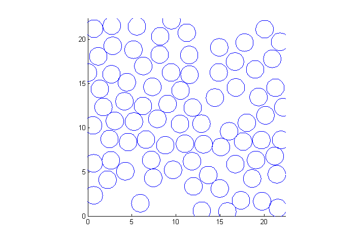
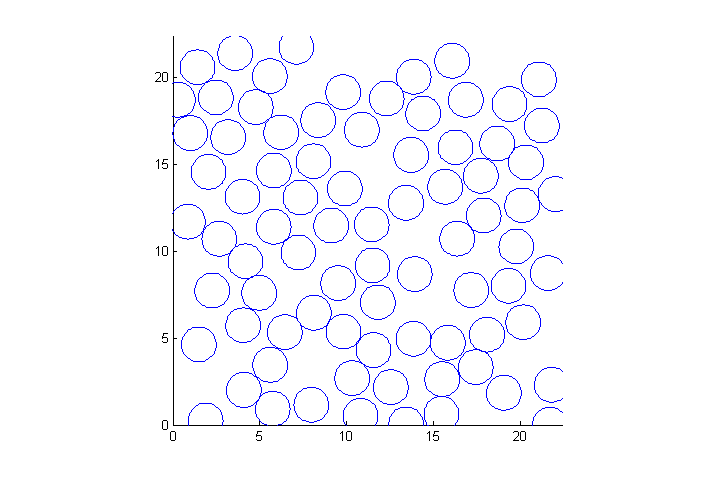
- In the command window type: mdNVE000 and then press enter. The code should run the default simulation of N=80, in a box with phi_set=.5 = 50% of the area covered by the disks, and an energy E=3. There should be an animation in the figure window. I find it useful to dock the figure window so that the command window and the figure are visible at the same time. As the code is running dots appear in the command window to indicate progress. Each dot is 10% of the simulation.
- Now run it again, but this type tic; mdNVE000; toc. The command tic; records the start time and toc displays the elapsed time in seconds. Record the time it takes and report it along with an error estimate using only significant figures in your report. Here is an similar example:
tic; override={'TT',10};mdNVE000; toc; clear('override');
..........Done.
Elapsed time is 0.321020 seconds.
Exercise II
Changing the default behavior:
In the command above notice the use of the cell-list variable override. A cell-list is a variable container in matlab. Cells can hold any objects including other cells. In this case override holds option pairs.
- Open mdNVE000.m by typing edit mdNVE000 in the command window. I find docking the editor window next to the figure with the command window below allows easy access to everything you need. In the file on line 41 the variable TT=500 is defined.
TT=500; % total simulation time
TT is the total simulation time. The simulation works by moving forward small steps at a time. For example, if a particle is a x=0 at the beginning of the simulation with a velocity of vx=.3 then a short time later it will move to a new location x_new=x_old+vx*dt. In this simulation the small time dt=.01 so the new x after one time step would be x=x+.3*.01=.003. This is a simplification if you are interested in the details look at An introduction to molecular dynamics in Matlab. Then TT=Nt*dt, where Nt is the total number of time steps. # To run the code with a different TT use override={'TT',20}. Notice the curly brackets and the single quotes for variable names. Only single quotes on the variable that changes so:
for nv=1:3; |override={'TT',200*nv}|;mdNVE000;end
will run three simulation with TT=200 then TT=400 then TT=600. Try running the simulation again with this command:
tic; override={'TT',20};mdNVE000; toc; clear('override');
This command tells the code to set TT=20. The override lasts as long a it is defined. In this case, we clear it at the end of the command, but if we wanted to do many runs with TT=20, we could leave it.
- Record the new execution time. Does it make sense? Here is mine:
tic; override={'TT',20};mdNVE000; toc; clear('override');
..........Done.
Elapsed time is 0.566075 seconds.
Exercise III
Conservation of Energy and More overrides:
You can override more than one variable: override={'TT',1000,'KE0',10}. Here it would increase the simulation time from the default 500 and change the initial total Kinetic Energy KE0 to 10. You can also add on to a previously defined override: override=[override,{'phi_set',.8}] Also change the initial density to 80% coverage. Notice the square bracket to concatenate. The order of the pairs does not matter, but they have to be pairs.
The simulation defines and saves a lot of information about the system. From the code here is a sample:
%% Save Variables
Ek=zeros(Nt,1);     % kinetic energy of particles
Ep=zeros(Nt,1);     % particle-particle potential energy
Ps=zeros(Nt,2,2);   % pressure tensor
if(saveall)
  xs=zeros(Nt,N);    % all particle x-positions
  ys=zeros(Nt,N);    % all particle y-positions
  vxs=zeros(Nt,N);   % all particle x-velocities
  vys=zeros(Nt,N);   % all particle y-velocities
end
- Using what we have learned run a simulation with KE0=1 and phi_set=.7.
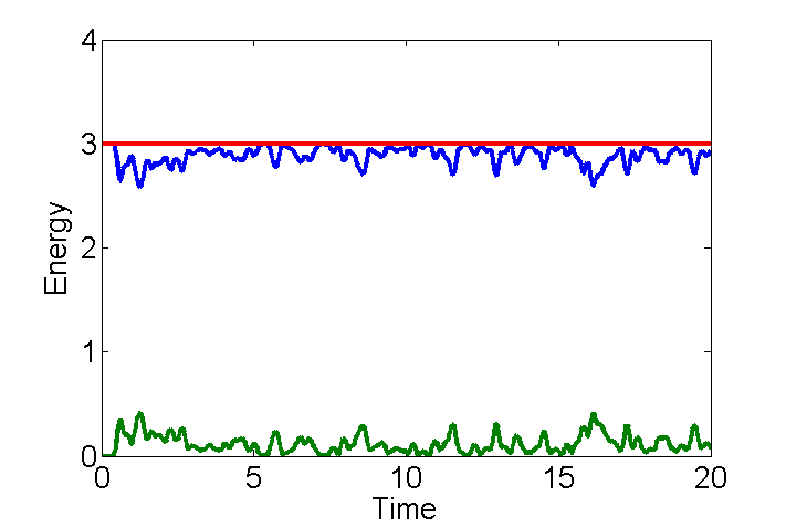
- Plot the kinetic energy Ek, and the potential energy Ep, and the total energy Ek + Ep as a function of time.
- To get the time right we need a time variable t=(1:Nt)*dt; The colon operator make a list from 1 to Nt the total number of steps (see line 77.) Ek and Ep are also 1 by Nt vectors. Here are the commands to make a nice plot. This one is shorter in time and at a different energy and density.
Plot KE and PE
t=(1:Nt)*dt;                         % make a time variable from dt to TT
plot(t,[Ek Ep Ek+Ep],'linewidth',3)  % concatenate variable to add to plot
set(gca,'fontsize',20);              % make font bigger
xlabel('Time')                       % axis labels
ylabel('Energy')
Exercise IV
Distributions.
- Plot the distribution of velocities for vx and vy separately. Is there a difference? Do you recognize the distribution? In matlab: [nn,bb]=hist(vxs(:),-.5:.1:.5);plot(bb,nn); will get you started. It produces a distribution plot. nn(p) contains the number of times vxs had a value between bb(p)-.1/2 and bb(p)+.1/2 where .1 is the bin size. vxs is matrix with size(vxs)=[Nt,N] so vxs(:) has size(vxs(:))=[1,Nt*N] puts all the data in one dimension.
- A bin size of 0.1 is not ideal. Try some other sizes. What bin size did you use? Why? What is the mean and std of the distribution?
- Assuming the distribution P(vx) is normal, use the mean and std to plot the limiting distribution along with the data. Make sure they are both normalized so the area under the distribution is 1. When nn is correctly normalized in matlab sum(nn)*binsize=1,
- For this section include in you report a single normalized plot of P(vx), P(vy), and an ideal normal distribution using the mean ans std of P(vx).
Exercise V
Units and area fraction (density)
In the computer there are no meters, so we are free to set the units however we like. For example the disks have a diameter of 2, but 2 "what?". Until we compare to something in the real world it could be  or
or  miles. For this simulation there are only 3 units length, mass, and time. One common way to deal with this is to measure everything in non-dimensional units. So we might measure distances in units of the particle diameter or the box size. We might get a time from the typical collision time
  . To connect to the real world we could use the particle area fraction, the total disk area divided by the box area:

In the code this determined by phi_set.
- Investigate what happens when you change phi_set with everything else the same. This is equivalent to changing the V in the NVE simulation. Show how the average Ek changes with density for 3 or 4 densities.
Exercise VI
Equation of state:
To non-dimensionalize the energy we need to include the pressure, which is conjugate to A=Lx*Ly or phi_set. Pressure is a measure of momentum flux so there are two ways momentum moves around. Particles carry momentum as they move and they exchange momentum when they collide.
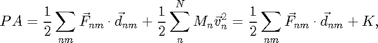
where  is a sum only over collision between
  and
and  ,
,  is the force between and and
  is the vector between and . The second term is the total kinetic energy
  . If there are no collisions the first term is zero and
 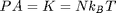 , the ideal gas law equation of state. Since we are trying to get rid of dimensional quantities, we will continue to use or Ek from the simulation. Then we can define the non-dimensional compressibility factor:
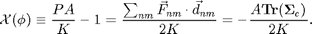
 is non-dimensional and depends only on a non-dimensional quantity the area fraction
  . In the simulation we measure the collisional pressure (stress) tensor
  as Ps. Momentum flux is a 2x2 tensor so the pressure tensor Ps has 4 components at each time step. We only need the isotropic pressure or the half of the trace of the tensor. The pressure we calculate in the code is the negative of the usual pressure.
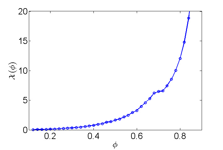
- Use the code to calculate
 for
for  with default conditions except for the box shape. If we want to get to high densities in such small systems we need to make sure the box fits a hexagonal pattern. So override={'phi_set',.1,'Gb',8/5/sqrt(3)}; Gb is the ratio of Lx/Ly. This will create a box which holds an exact 8x10 hexagonal array. Use enough values of phi_set to get a good idea of what is going on, and give a short discussion of the plot of
  vs . Include a description of what is happening around
  .
.
If you need some help here is script to do the measurements.
if(~exist('MDLabIdata.mat','file'))  % only run first time
  Nv=40;                  % number of points between .1 and .9 ~10 min
  phlist=(1:Nv)/Nv*.8+.1; % list of 40 numbers between .1 and .9
  Pc=zeros(1,Nv);         % store average Pc for each run
  Ks=zeros(1,Nv);         % " Ek for each run
  Es=zeros(1,Nv);         % " total for each run (check for conservation)
  for nv=1:Nv;            % loop
    override={'phi_set',phlist(nv),'Gb',8/5/sqrt(3)};    % set overrides
    mdNVE000;                                            % run simulation
    % find average value over last half of sim
    Pc(nv)=-mean(Ps(end/2:end,1,1)+Ps(end/2:end,2,2))/2; % average collisional
    Ks(nv)=mean(Ek(end/2:end));                          % kinetic
    Es(nv)=mean(Ek(end/2:end)+Ep(end/2:end));            % total for check
    % visual feedback
    figure(2);
    plot(phlist(1:nv),Lx*Ly*Pc(1:nv)./Ks(1:nv));
    drawnow;
    figure(1);
  end
  save('MDLabIdata.mat');     % save for later
else
  load('MDLabIdata.mat');     % load second time around
end

% nice plot:
plot(phlist,Lx*Ly*Pc./Ks,'o-','linewidth',2);
axis([.1 .9 0 20])
set(gca,'fontsize',20);
xlabel('$$\phi$$','interpreter','latex');
ylabel('$$\mathcal{X}(\phi)$$','interpreter','latex');
m-files
- MDLabI.zip All files in one zip file.
- MDLabI.m Instruction and description of Molecular Dynamics Lab. I
- MDLabI.pdf (pdf version).
- mdNVE000.m NVE simulator.
- plotNCirc.m Helper function to draw circles.
Data files
- MDLabIdata.mat Data file for compressibility factor
