Molecular Dynamics Simulation

An introduction to soft-particle Molecular Dynamics (MD) simulation. This file is also a working MD simulator. A companion file introMDpbc.m is also available with fewer comments.

Contents

Theory I: Solving Newtons Laws for collection of particles

A Molecular Dynamics (MD) simulation is a computer simulation of Newton's Laws for a collection of $N$ particles. The $n$-th particle at initial position $\vec{x}_n(0)$ with velocity $\vec{v}_n(0)$ moves according to Newton's Law:

$M_n\frac{d^2}{d t^2}\vec{x}_n(t)=\vec{F}_{n}(t)= \sum_{m=1}^N \vec{F}_{nm}(t)+\vec{F}_n^e(t),\;\;\;\;\;\;[1]$

where $M_n$ is the mass of particle $n$, $\vec{F}_{n}(t)$ is the force on particle $n$, $\vec{F}_{nm}(t)$ is the force on particle $n$ from particle $m$, and $\vec{F}_n^e(t)$ is the sum of all external forces. For this introduction, we assume that the force is obtained from a scalar potential $\Phi(\vec{x}_n)$ such that

$\vec{F}_{nm}= -\frac{\partial}{\partial\vec{x}_n} \Phi(\vec{x}_m,\vec{x}_n). \;\;\;\;\;\;[2]$

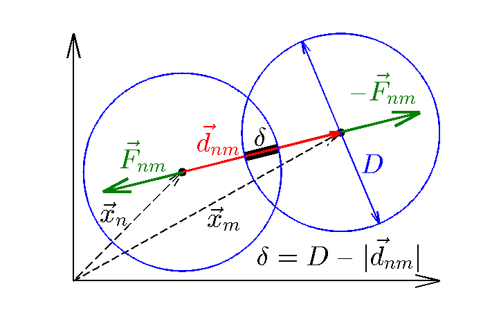
Figure 1: Diagram defining particle-particle interaction variables.

MDfigures(1);

We will further assume the particles are disks with a simple harmonic potential:

$\Phi(\vec{x}_m,\vec{x}_n) = \Phi(|\vec{x}_m-\vec{x}_n|) = \Phi(d_{nm})=\frac{1}{2}K(D-d_{nm})^2=\frac{1}{2}K\delta^2, \;\;\;\;\;\;[3a]$

where

$\vec{d}_{nm}=\vec{x}_m-\vec{x}_n \;\;\;\;\;\;[3b]$

is the vector pointing from the center of particle $n$ to the center of particle $m$ and

$d_{nm}=|\vec{d}_{nm}|; \;\;\;\;\;\;[3c]$

$K$ is a material constant that determines how hard the material is, $D$ is the particle diameter, and

$\delta=D-|\vec{d}_{nm}| \;\;\;\;\;\;[3d]$

is the particle overlap. (See Figure 1.) Differentiating the potential, the force

$\vec{F}_{nm}=-K \delta\hat{d}_{nm}. \;\;\;\;\;\;[3e]$

The direction of the force is opposite to the unit vector $\hat{d}_{nm}$ pointing from particle $n$ to $m$, which pushes the particles apart. From Newton's third law the force on particle $m$ from $n$ is

$\vec{F}_{mn}=-\vec{F}_{nm}. \;\;\;\;\;\;[3f]$

In this introduction we use a contact force, which only acts when the particles are in contact. That is, the force is zero if

$\delta<=0. \;\;\;\;\;\;[3g]$

Simple Molecular Dynamics Simulation

introMDpbc.m contains the same code without the explanation:

Experimental Parameters (particle)

Here we define all of the particle parameters needed to determine the forces between particle pairs:

N=80;  % number of particles
D=2;   % diameter of particles
K=100; % force vector n<-m Fnm=-K*(D/|dnm|-1)*dnm, where vect dnm=Xm-Xn
M=3;   % mass of particles

Experimental Parameters (space-domain)

This simulation uses a periodic domain. In a periodic domain there are copies or images of each particle separated by $L_x$ and $L_y$ such that for each particle a positions $(x,y)$ there are also particles at

$(x+k L_x,y+l L_y),$

for all integers $k$ and $l$. In the main simulation box $k=0$ and $l=0$. For this simulation we need the distance between all particle pairs, but since we have a short range potential [3g] we only need the nearest image distance. This calculation is done below in the main loop.

Here we define parameters needed to determine the space-domain for the particles in a periodic box of size Lx by Ly.

Lx=10*D;  % size of box
Ly=10*D;

Experimental Parameters (initial conditions)

We choose random velocities with the property that the total kinetic energy: M/2*sum(vx.^2+vy.^2)=KEset.

KEset=5;  % initial total Kinetic Energy (KE)

Experimental Parameters (time-domain)

The time-domain is from 0 to TT.

TT=1;    % total simulation time (short for demo).

Display Parameters

This section controls the simulation plotting animation

demo=true;       % true for this demo
plotit=false;    % plot ? off for this demo
Nplotskip=50;    % number of time steps to skip before plotting

Theory II: Numeric integration of Newton's laws Part I

To solve [1] we first rewrite it as two first-order equations:

$\begin{array}{lcl} \displaystyle \frac{d}{dt}\vec{x}_n(t) & = & \vec{v}_n(t).\\[13pt] \displaystyle \frac{d}{dt}\vec{v}_n(t) & = & \vec{F}_n(t)/M_n.\\ \end{array} \;\;\;\;\;\;[4]$

When solving [4] numerically, time is broken up into discrete steps of size $\Delta t$ (i.e., $t=k\Delta t$, where k is an integer). If $\Delta t$ is small we can approximate [4] with:

$\begin{array}{lcl} \left[ \vec{x}_n\left( (k+1)\Delta t \right) -\vec{x}_n(k\Delta t) \right]/\Delta t & \simeq & \vec{v}_n(k\Delta t).\\[10pt] \left[ \vec{v}_n\left( (k+1)\Delta t \right) -\vec{v}_n(k\Delta t) \right]/\Delta t & \simeq & \vec{F}_n(t)/M_n.\\ \end{array} \;\;\;\;\;\;[5]$

Solving for the later times $(k+1)\Delta t$ in terms of earlier times $k\Delta t$:

$\begin{array}{lclcl} \vec{x}_n^{(k+1)} & \equiv & \vec{x}_n\left( (k+1)\Delta t \right) & \simeq & \vec{x}_n^{(k)}+\vec{v}_n^{(k)}\Delta t\\[10pt] \vec{v}_n^{(k+1)} & \equiv & \vec{v}_n\left( (k+1)\Delta t \right) & \simeq & \vec{v}_n^{(k)}+\vec{F}_n^{(k)}/M_n\Delta t\\ \end{array} \;\;\;\;\;\;[6]$

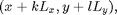
Equation [6] discovered by L. Euler is called the Euler Method and could be used to integrate the system to get the new positions $\vec{x}_n^{(k+1)}$ and velocities $\vec{v}_n^{(k+1)}$ from the old positions $\vec{x}_n^{(k)}$, velocities $\vec{v}_n^{(k)}$, and forces $\vec{F}_n^{(k)}(\vec{x}_n^{(k)})$, which only depends on $\vec{x}_n^{(k)}$. However [6] is not recommended. If we use [6] the energy of the system will grow without bounds as seen in Figure 2. To make a useful integration scheme we can change the order of integration. If we calculate $\vec{v}_n^{(k+1)}$ first we can use it to calculate $\vec{x}_n^{(k+1)}$. These equation are an enhanced version of Euler's method called the Semi-implicit Euler Method:

$\begin{array}{lcl} \vec{v}_n^{(k+1)} &\simeq& \vec{v}_n^{(k)}+\vec{F}_n^{(k)}/M_n\Delta t.\\[10pt] \vec{x}_n^{(k+1)} &\simeq& \vec{x}_n^{(k)}+\vec{v}_n^{(k+1)}\Delta t.\\ \end{array} \;\;\;\;\;\;[7]$

Figure 2 compares an Euler simulation from eulerMDpbc.m with an semi-implicit Euler simulation from eEulerMDpbc.m. The semi-implicit Euler method is the simplest example of a general method called Symplectic Integration, which is designed to conserve energy.

Figure 2: Euler vs. Semi-implicit Euler Integration.

The following code is used to produce figure 2. External files eulerMDpbc.m and eEulerMDpbc.m are used.

KE=5;                                % initial Kinetic Energy
Ts=100;                              % total simulation time
[Ek Ep]=eulerMDpbc(10,KE,Ts,false);  % 10 particle--Euler integration
eTe=Ek+Ep;                           % save total energy for Euler;
[Ek Ep]=eEulerMDpbc(10,KE,Ts,false); % 10 particle--Semi-implicit Euler
eTse=Ek+Ep;                          % save total energy for semi-implicit Euler
Nt=length(Ek);                       % number of time steps
t=(0:Nt-1)/Nt*Ts;                    % simulation time
fs=25;
plot(t,eTe,t,eTse,'r','linewidth',2);  % plot total energy
axis([0 Ts 0 inf]);
set(gca,'fontsize',fs);
xlabel('Time');
ylabel('Total Energy');
text(80,eTe(fix(90/Ts*Nt)),'Euler',...
  'color','b','fontsize',fs,'horizontal','right');
text(80,.9*KE,'Semi-implicit Euler',...
  'color','r','fontsize',fs,...
  'horizontal','right','vertical','top');

Theory II: Numeric integration of Newton's laws Part II

It is clear that energy conservation is poor using the (blue) Euler method. In principle Equation [7] could be used for simple MD simulations. However, both methods are only accurate to first order in $\Delta t$, and this limits the usefulness of the semi-implicit Euler method.

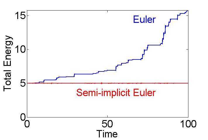
In this introduction we use a Symplectic Integrator with errors proportional to $(\Delta t)^2$ and good energy conservation due to L. Verlet called Velocity Verlet integration. The main drawback of the semi-implicit Euler method the error is proportional to $\Delta t$. Since we used dt=0.01, we can expect errors of order 1% (see Figure 3). Sometimes that is not sufficient. One option is to decrease dt, but the drawback is that the simulation time is increase proportionally. So with dt=0.01/100=0.0001 semi-implicit Euler would give error of order 0.01% the simulation time would increase by a factor of 100. To overcome this deficiency Verlet devised a different integration scheme based on a second order approximation to [4] as follows:

$\begin{array}{lcll} \vec{x}_n^{(k+1)} &\simeq& \vec{x}_n^{(k)}+ \vec{v}_n^{(k)}\Delta t+ \frac{1}{2}\vec{a}_n^{(k)}(\Delta t)^2. &\;\;\;\;\;\;[8]\\[10pt] \displaystyle \vec{a}_n^{(k+1)} &=& \displaystyle \frac{1}{M_n}\sum_{m=1}^N \vec{F}_{nm}(|\vec{x}_m^{(k+1)}-\vec{x}_n^{(k+1)}|) &\;\;\;\;\;\;[9]\\[20pt] \vec{v}_n^{(k+1)} &\simeq& \vec{v}_n^{(k)}+ \frac{1}{2}(\vec{a}_n^{(k+1)}+\vec{a}_n^{(k)})\Delta t. &\;\;\;\;\;\;[10]\\ \end{array}$

Figure 3: Velocity Verlet vs. Semi-implicit Euler Integration.

The following code is used to produce figure 3. External files verletMDpbc.m and eEulerMDpbc.m are used.

KE=5;                                 % initial Kinetic Energy
Ts=100;                               % total simulation time
[Ek Ep]=verletMDpbc(10,KE,Ts,false);  % 10 particle--Verlet integration
eTv=Ek+Ep;                            % save total energy for Verlet;
Nt=length(Ek);                        % number of time steps
t=(0:Nt-1)/Nt*Ts;                     % simulation time
fs=25;
plot(t,eTv,t,eTse,'r','linewidth',2); % plot total energy
hold on;
plot(t,[0*t+1.01*KE;0*t+.99*KE],'r--','linewidth',2);  % 1% error
plot([73 85],[1.014 1]*KE,'linewidth',2);
hold off;
axis([0 Ts 5*(1+[-.02 .0201])]);
set(gca,'fontsize',fs);
xlabel('Time');
ylabel('Total Energy');
text(50,1.014*KE,'Velocity Verlet',...
  'color','b','fontsize',fs,'horizontal','center');
text(50,.988*KE,'Semi-implicit Euler \pm 1%',...
  'color','r','fontsize',fs,...
  'horizontal','center','vertical','top');

Figure 3: Velocity Verlet vs. Semi-implicit Euler Integration (caption).

Figure 3 shows the total energy over time for a 10 particle system using the Semi-implicit Euler integration method from [7] (red) and Velocity Verlet from [8-10] (blue). Red dashed lines show a range of $\pm 1\%$. The error for the Velocity Verlet is $\approx 100$ times smaller.

Simulation Parameters

Regardless of the integration method $\Delta t$ (dt in code) must be determined. Here we use a fixed time step dt=0.01 $\simeq\sqrt{M/K}/20$. The total number of time steps Nt is determined from the total simulation time TT.

dt=1e-2;       % integration time step
Nt=fix(TT/dt); % number of time steps

Initial Conditions (Positions)

The particles need to be placed in the box with minimal overlap to avoid excess potential energy at the beginning of the simulation. For moderately dense systems a square grid can be used. The matlab command ndgrid creates D spaced points on a grid inside of the Lx by Ly box. randperm randomly chooses N positions from all numel(x) available locations. The final result is a pair of matlab vectors x and y each with size(x)=[1,N] that represents $\vec{x}_n^{(k)}$ at each time $k\Delta t$. Here, for the initial conditions before the simulation starts $k=0$. In the code $k$ is represented in matlab as nt, the time step number.

[x y]=ndgrid(D/2:D:Lx-D/2,D/2:D:Ly-D/2); % place particles on grid
ii=randperm(numel(x),N);                 % N random position on grid
x=x(ii);                                 % set x-positions
y=y(ii);                                 % set y-positions

Initial Conditions (Velocities)

The velocities vx and vy each with size(vx)=[1,N] represent $\vec{v}_n^{(k)}$ at time $k\Delta t$. Here, for the initial conditions before the simulation starts $k=0$. The velocities are chosen randomly from a normal distribution using randn. The mean velocity is removed to avoid center of mass drift. The variance of the distribution is set so that the total kinetic energy: M/2*sum(vx.^2+vy.^2)=KEset.

vx=randn(1,N)/3;  % normal (Maxwell) distribution of velocities
vy=randn(1,N)/3;

vx=vx-mean(vx);   % remove center of mass drift
vy=vy-mean(vy);

tmp=sqrt(2*KEset/M/sum((vx.^2+vy.^2)));  % set Kinetic energy
vx=vx*tmp;
vy=vy*tmp;

Initial Conditions (Accelerations)

The accelerations from the $k-1$ previous time step is need for Verlet's second order integration scheme.

ax_old=0*x;       % need initial condition for velocity Verlet integration
ay_old=0*y;

Save variables

List of quantities to be saved at each time step.

Ek=zeros(Nt,1);    % Kinetic Energy
Ep=zeros(Nt,1);    % particle-particle potential
xs=zeros(Nt,N);    % x-position
ys=zeros(Nt,N);    % y-position
vxs=zeros(Nt,N);   % x-velocity
vys=zeros(Nt,N);   % y-velocity

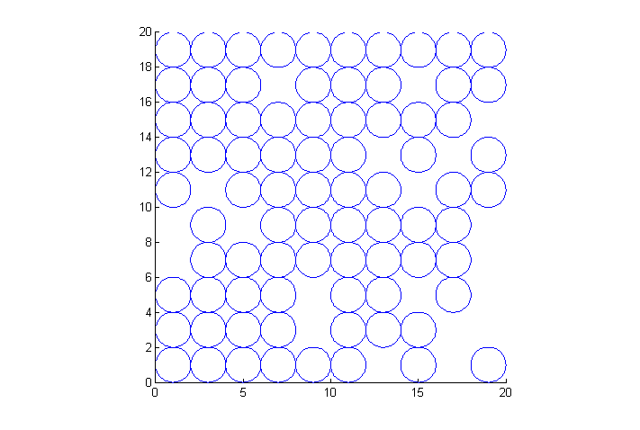
Figure 3: Setup Plotting

Here we use an external function plotNCirc.m to create an animation of the simulations progress. plotNCirc returns an array of handles h to a rectangle object for each of the N particles. Matlab rectangles contain a curvature property with turns them into circles. The handles are used later to animate the particle positions. An example initial condition is shown here.

NB: periodic images of particles are not shown

if(plotit || demo)            % only if plotit true
  clf;                        % clear figure
  h=plotNCirc(x,y,D,'none');  % plot particles no color; store handle h
  axis('equal');              % square pixels
  axis([0 Lx 0 Ly]);          % piloting range
end

Main Loop

In the main loop the simulation steps through Nt time steps, advancing time, the particle positions, forces, and velocities. Comments refer back to sections and equations above.

for nt=1:Nt

  % plot particles
  if(plotit && rem(nt-1,Nplotskip+1)==0)  % nt-1 divides Nplotskip+1
    xp=mod(x,Lx);
    yp=mod(y,Ly);
    for np=1:N
      set(h(np),'Position',[xp(np)-.5*D yp(np)-.5*D D D]); % update handle
    end
    drawnow;
  end

  x=x+vx*dt+ax_old*dt^2/2;  % first step in Verlet integration eq.[8]
  y=y+vy*dt+ay_old*dt^2/2;

  % position dependent calculations
  xs(nt,:)=x;                         % save positions
  ys(nt,:)=y;

  % Force between particles eq. [9] and [3a-g]
  Fx=zeros(1,N);                      % zero forces
  Fy=zeros(1,N);

  for nn=1:N                       % check particle n
    for mm=nn+1:N                  % against particle m from n+1->N
      dy=y(mm)-y(nn);              % [3b] y-comp dnm vector from from n->m
      dy=dy-round(dy/Ly)*Ly;       % closest periodic image
      if(abs(dy)<D)                % [3g] y-distance close enough?
        dx=x(mm)-x(nn);            % [3b] x-comp dnm vector from from n->m
        dx=dx-round(dx/Lx)*Lx;     % closest periodic image
        dnm=dx.^2+dy.^2;           % [3c] squared distance between n and m
        if(dnm<D^2)                % [3g] overlapping?
          dnm=sqrt(dnm);           % [3c] distance
          F=-K*(D/dnm-1);          % [3d-e] force magnitude
          Fx(nn)=Fx(nn)+F.*dx;     % [9,3e] accumulate x force on n
          Fx(mm)=Fx(mm)-F.*dx;     % [9,3ef] x force on m (equal opposite)
          Fy(nn)=Fy(nn)+F.*dy;     % [9,3e] accumulate y force on n
          Fy(mm)=Fy(mm)-F.*dy;     % [9,3ef] y force on m (equal opposite)
          Ep(nt)=Ep(nt)+(D-dnm).^2;% [3a] particle-particle potential I
        end
      end
    end
  end
  Ep(nt)=K/2*Ep(nt);        % eq [3a] particle particle potential II

  ax=Fx./M;                 % eq [9] calc a from F=Ma
  ay=Fy./M;

  vx=vx+(ax_old+ax)*dt/2;   % eq [10] second step in Verlet integration
  vy=vy+(ay_old+ay)*dt/2;

  % velocity dependent calculations
  Ek(nt)=M*sum((vx.^2+vy.^2))/2; % Kinetic energy
  vxs(nt,:)=vx;                  % save velocities
  vys(nt,:)=vy;

  ax_old=ax;                % need for eqs [8-10] save for next step
  ay_old=ay;
end

m-files

Published with MATLAB® 7.14